 BeamZ
Four-channel WDM inverse design in BeamZ
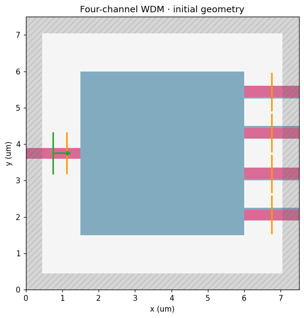
Route 1270, 1290, 1310, and 1330 nm into four output guides. This is a 2D lossless silicon/air model, not a full silicon-on-insulator stack. All geometry uses metres and all inverse-design features live in beamz.optimization.
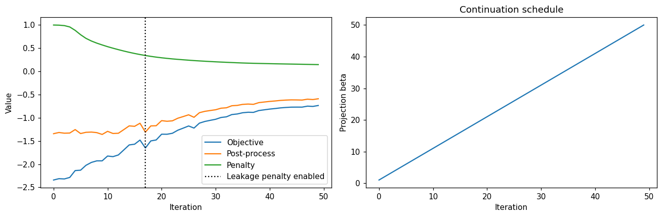
The optimization uses one broadband input, five training frequencies per channel, a smooth minimum across channels, an erosion/dilation penalty on the parameters, and 50 Adam updates. Beta increases from 1 to 50; leakage weight switches from 0 to 1 at zero-based step 17.
Computation choices: BeamZ uses a uniform 50 nm mesh and a 6 ps run; spectral gradient evaluations check forward and adjoint decay. Full autodiff differentiates the configured finite window; a longer-duration verification follows optimization. Gaussian bandwidth, Yee interpolation, filtering discretization, and mode normalization follow BeamZ conventions. These settings demonstrate the workflow and do not establish fabrication readiness.
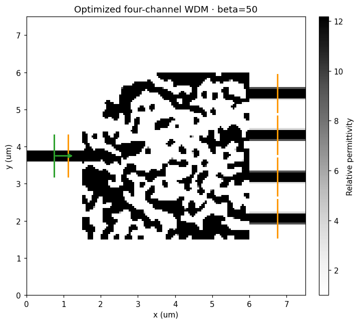
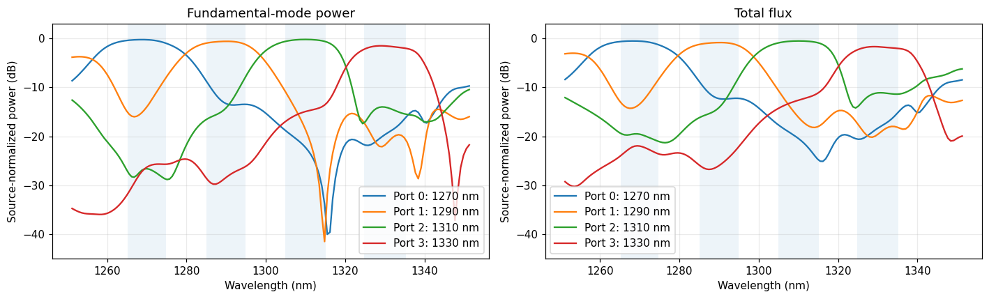
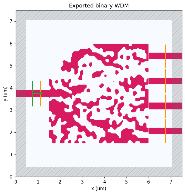
Result from this execution: all 50 updates completed. The continuous 50 nm model shows four separated passbands, but the binary export is sensitive to rerasterization: at 30 nm its desired-channel transmissions are 41.4%, 45.2%, 42.5%, and 15.1%. The 6 and 12 ps values agree closely. This example validates the optimization workflow; it does not establish a mesh-converged device. The source aperture is 1.125 µm.
Setup
Use the repository's Python environment (uv sync --extra dev) as the notebook kernel. Everything runs locally through JAX. The execution below saves optimizer history and verification arrays under results/topology_examples/topology_wdm_4channel/.
from pathlib import Path
import time, json, gc
import numpy as np
import jax
import jax.numpy as jnp
from jax.scipy.special import logsumexp
import matplotlib.pyplot as plt
from IPython.display import display, Markdown
from beamz import (LIGHT_SPEED, Design, Material, Rectangle, Simulation, ModeSource,
                   ModeMonitor, FieldMonitor, FluxMonitor, ModeSpec, GaussianPulse, PML)
import beamz.optimization as opt

um = 1e-6
wavelengths_design = np.array([1.270, 1.290, 1.310, 1.330])*um
frequencies_design = LIGHT_SPEED / wavelengths_design
frequency = frequencies_design.mean()
fwidth = np.ptp(frequencies_design)
channel_width = abs(np.diff(frequencies_design).mean()) / 2
channel_frequencies = np.array([np.linspace(f-channel_width/2, f+channel_width/2, 5)
                                for f in frequencies_design])
training_frequencies = channel_frequencies.ravel()
output_y = (1.5 + np.linspace(.5625, 3.9375, 4))*um


root=next(p for p in [Path.cwd(),*Path.cwd().parents] if (p/"pyproject.toml").exists())
artifacts=root/"results/topology_examples/topology_wdm_4channel"
artifacts.mkdir(parents=True,exist_ok=True)
plt.rcParams.update({"figure.dpi":110,"font.size":10})
print("JAX:",jax.__version__,"backend:",jax.default_backend())
JAX: 0.9.0 backend: cpu
Geometry, modal objective, and schedules
Rows of the power matrix represent output ports; columns represent wavelength bands. For each output, subtract the average leakage from the other three bands, then take -logsumexp(-metrics) with temperature 1. Its absolute value can be negative; it is an optimization score, not transmission efficiency.
The objective uses source-normalized modal power. An additional input monitor supports separately reported incident-normalized verification. The native tm label in BeamZ selects the 2D Ez field polarization.
def make_wdm(resolution=50e-9, duration=6e-12, backend="adjoint", grouping="frequency"):
    air, silicon = Material(1), Material(3.49**2)
    geometry = Design(width=7.5*um, height=7.5*um, material=air)
    geometry += Rectangle(position=(0,3.6*um), width=1.5*um, height=.3*um, material=silicon)
    for y in output_y:
        geometry += Rectangle(position=(6*um,y-.15*um), width=1.5*um, height=.3*um, material=silicon)
    mode = ModeSpec(num_modes=1, polarization="tm")
    source = ModeSource(center=(.75*um,3.75*um,0),size=(0,1.125*um,um),direction="+",
        mode_spec=mode, source_time=GaussianPulse(freq0=frequency,fwidth=fwidth,offset=5/(2*np.pi)))
    outputs = [ModeMonitor(center=(6.75*um,y,0),size=(0,1.0125*um,um),freqs=training_frequencies,
                mode_spec=mode,name=f"mode_{i}") for i,y in enumerate(output_y)]
    incoming = ModeMonitor(center=(1.125*um,3.75*um,0),size=(0,1.125*um,um),
                           freqs=training_frequencies,mode_spec=mode,name="input")
    simulation = Simulation(design=geometry,resolution=resolution,run_time=duration,polarization="tm",
        sources=[source],monitors=[*outputs,incoming],boundaries=[PML(thickness=.45*um,formulation="cpml")])
    region = opt.TopologyDesignRegion(center=(3.75*um,3.75*um,0),size=(4.5*um,4.5*um,np.inf),
        pixel_size=resolution,eps_bounds=(1,3.49**2),transformations=[opt.FilterProject(radius=.1*um,beta=1)],
        penalties=[opt.ErosionDilationPenalty(length_scale=.1*um,beta=10)],penalty_input="parameters")
    return opt.InverseDesign(simulation,region,output_monitor_names=[f"mode_{i}" for i in range(4)],
        gradient_backend=backend,adjoint_source_grouping=grouping,checkpoint_interval=128)


def channel_powers(data):
    # Rows are output ports; columns are wavelength channels, five frequencies each.
    return jnp.stack([jnp.abs(data[f"mode_{i}"].amps.sel(direction="+",mode_index=0).values.reshape(4,5))**2
                      for i in range(4)]).mean(axis=-1)


def post_process(data, leak_weight=0.0):
    power = channel_powers(data)
    desired = jnp.diag(power)
    leakage = (power.sum(axis=1)-desired)/3
    return -logsumexp(-(desired-leak_weight*leakage))

schedule = opt.OptimizationSchedule(beta=opt.LinearSchedule(1,50,50),
    objective_kwargs={"leak_weight":opt.StepSchedule(0,1,17)})

design=make_wdm()
params0=design.design_region.initial_parameters
print("Design parameters:",params0.shape,params0.size)
print("Training frequencies:",len(training_frequencies),"timesteps:",len(design.simulation.time))
fig,ax=design.initial_simulation.plot(figsize=(7,6))
ax.set_title("Four-channel WDM · initial geometry")
plt.show()
Design parameters: (90, 90) 8100
Training frequencies: 20 timesteps: 51391
Independent gradient and source-grouping checks
On a 75 nm mesh, compare full autodiff, independent-frequency adjoints, and broadband source-basis adjoints at the same perturbed parameters and scheduled settings. A directional finite difference checks the full objective independently.
BeamZ's optional auto strategy factors the actual frequency-dependent source profiles into a smaller spatial basis, accepting a reduction only when every normalized source is reconstructed within 1e-7. It retains complex spectral weights and measured pulse normalization, with an independent-frequency fallback. This avoids assuming a mode profile is frequency-independent.
check=make_wdm(resolution=75e-9,backend="autodiff")
probe=check.design_region.initial_parameters+.015*np.random.default_rng(7).normal(size=check.design_region.params_shape)
settings=schedule.values(20)
values,gradients,timings,diagnostics={},{},{},{}
for label,backend,grouping in [("autodiff","autodiff","frequency"),("frequency","adjoint","frequency"),("auto","adjoint","auto")]:
    candidate=check if label=="autodiff" else check.updated_copy(gradient_backend=backend,adjoint_source_grouping=grouping)
    fn=candidate.make_objective_fn(post_process,**settings)
    started=time.perf_counter()
    value,gradient=jax.value_and_grad(fn)(probe)
    gradients[label]=np.asarray(gradient)
    values[label]=float(value)
    timings[label]=time.perf_counter()-started
    if backend=="adjoint":diagnostics[label]=candidate.gradient_diagnostics
    print(label,"score",values[label],"seconds",timings[label],diagnostics.get(label,{}),flush=True)
gradient_errors={name:float(np.linalg.norm(g-gradients["autodiff"])/np.linalg.norm(gradients["autodiff"])) for name,g in gradients.items()}
direction=gradients["autodiff"]/np.linalg.norm(gradients["autodiff"])
fn=check.make_objective_fn(post_process,**settings)
h=.01
finite_difference=float((fn(probe+h*direction)-fn(probe-h*direction))/(2*h))
np.testing.assert_allclose(finite_difference,np.sum(gradients["autodiff"]*direction),rtol=.01,atol=1e-6)
assert max(gradient_errors.values())<.005
print("Relative gradient errors:",gradient_errors,"directional finite difference:",finite_difference)
del check,candidate,fn,gradients
jax.clear_caches();gc.collect()
autodiff score -2.417819023132324 seconds 22.110200957977213 {}
frequency score -2.417819023132324 seconds 194.67079983407166 {'terminal_field_ratio': 4.382339682251768e-07, 'decay_tolerance': 0.0001, 'adjoint_solves': 20, 'source_grouping': 'frequency', 'adjoint_terminal_field_ratios': (3.071326500503346e-05, 9.830492672335822e-06, 1.7653193935984746e-05, 8.878190783434547e-06, 2.360725193284452e-05, 1.6110636352095753e-05, 2.4313700123457238e-05, 1.9657851225929335e-05, 1.5726094716228545e-05, 2.414094160485547e-05, 1.9379991499590687e-05, 2.333591146452818e-05, 2.0966350348317064e-05, 1.1841348168672994e-05, 2.4600880351499654e-05, 1.755172161210794e-05, 2.401211895630695e-05, 2.1245694370009005e-05, 1.1032696420443244e-05, 1.4613307939725928e-05), 'adjoint_timesteps': (34261, 34261, 34261, 34261, 34261, 34261, 34261, 34261, 34261, 34261, 34261, 34261, 34261, 34261, 34261, 34261, 34261, 34261, 34261, 34261), 'stored_design_dft_values': 74420}
auto score -2.417819023132324 seconds 198.08365995797794 {'terminal_field_ratio': 4.382339682251768e-07, 'decay_tolerance': 0.0001, 'adjoint_solves': 12, 'source_grouping': 'broadband_basis', 'source_basis_rank': 12, 'source_reconstruction_error': 8.104715908720145e-08, 'active_frequencies': 20, 'adjoint_terminal_field_ratios': (3.528527304297313e-05, 1.2401308595144656e-05, 1.7008251234074123e-05, 1.8966433344758116e-05, 2.6738709493656643e-05, 1.596302718098741e-05, 2.1747420760220848e-05, 3.006366932822857e-05, 2.4821179977152497e-05, 2.7630771000985987e-05, 1.7224763723788783e-05, 1.3552800737670623e-05), 'adjoint_timesteps': (34261, 34261, 34261, 34261, 34261, 34261, 34261, 34261, 34261, 34261, 34261, 34261), 'stored_design_dft_values': 74420}
Relative gradient errors: {'autodiff': 0.0, 'frequency': 2.60916531260591e-05, 'auto': 2.764066266536247e-05} directional finite difference: 1.7119646072387695
1399
Select and profile the training backend
Use the gradient-check timings to select a backend, then measure its cold and warmed gradient cost on the training mesh. Full autodiff can be faster for this modest 2D grid; the spectral adjoint offers different memory scaling. All routes use the same objective and schedules. Coarse timings are a heuristic, not a universal hardware benchmark.
chosen=min(timings,key=timings.get)
backend="autodiff" if chosen=="autodiff" else "adjoint"
grouping="auto" if chosen=="auto" else "frequency"
design=design.updated_copy(gradient_backend=backend,adjoint_source_grouping=grouping)
fn=design.make_objective_fn(post_process,**schedule.values(0))
elapsed=[]
for repeat in range(2):
    start=time.perf_counter()
    value,gradient=jax.value_and_grad(fn)(params0)
    np.asarray(gradient)
    elapsed.append(time.perf_counter()-start)
profile={"coarse_seconds":timings,"coarse_adjoint_diagnostics":diagnostics,
         "training_first_seconds":elapsed[0],"training_warm_seconds":elapsed[1]}
print("Selected backend:",chosen,"training profile:",profile,flush=True)
Selected backend: autodiff training profile: {'coarse_seconds': {'autodiff': 22.110200957977213, 'frequency': 194.67079983407166, 'auto': 198.08365995797794}, 'coarse_adjoint_diagnostics': {'frequency': {'terminal_field_ratio': 4.382339682251768e-07, 'decay_tolerance': 0.0001, 'adjoint_solves': 20, 'source_grouping': 'frequency', 'adjoint_terminal_field_ratios': (3.071326500503346e-05, 9.830492672335822e-06, 1.7653193935984746e-05, 8.878190783434547e-06, 2.360725193284452e-05, 1.6110636352095753e-05, 2.4313700123457238e-05, 1.9657851225929335e-05, 1.5726094716228545e-05, 2.414094160485547e-05, 1.9379991499590687e-05, 2.333591146452818e-05, 2.0966350348317064e-05, 1.1841348168672994e-05, 2.4600880351499654e-05, 1.755172161210794e-05, 2.401211895630695e-05, 2.1245694370009005e-05, 1.1032696420443244e-05, 1.4613307939725928e-05), 'adjoint_timesteps': (34261, 34261, 34261, 34261, 34261, 34261, 34261, 34261, 34261, 34261, 34261, 34261, 34261, 34261, 34261, 34261, 34261, 34261, 34261, 34261), 'stored_design_dft_values': 74420}, 'auto': {'terminal_field_ratio': 4.382339682251768e-07, 'decay_tolerance': 0.0001, 'adjoint_solves': 12, 'source_grouping': 'broadband_basis', 'source_basis_rank': 12, 'source_reconstruction_error': 8.104715908720145e-08, 'active_frequencies': 20, 'adjoint_terminal_field_ratios': (3.528527304297313e-05, 1.2401308595144656e-05, 1.7008251234074123e-05, 1.8966433344758116e-05, 2.6738709493656643e-05, 1.596302718098741e-05, 2.1747420760220848e-05, 3.006366932822857e-05, 2.4821179977152497e-05, 2.7630771000985987e-05, 1.7224763723788783e-05, 1.3552800737670623e-05), 'adjoint_timesteps': (34261, 34261, 34261, 34261, 34261, 34261, 34261, 34261, 34261, 34261, 34261, 34261), 'stored_design_dft_values': 74420}}, 'training_first_seconds': 111.67431387491524, 'training_warm_seconds': 139.89644858404063}
Optimize and demonstrate exact schedule continuation
The linear schedule has a fixed 50-update horizon, independent of how many updates are requested before a pause. Stop at 25, restore the saved Adam state, then finish to 50. Each callback records the actual beta and leakage weight, plus decay ratios and solve counts when using the spectral backend. No design symmetry is imposed: the reference assigns distinct wavelengths to distinct output ports.
optimizer = opt.AdamOptimizer(design=design, learning_rate=.1, schedule=schedule,
    objective_id="reference-wdm-four-channel-v1")
checkpoint = artifacts / "history.npz"
started = time.perf_counter()
progress_rows = []
def report(result):
    h = result.history[-1]
    row = dict(step=h.step, score=h.objective_before, post=h.post_process_val,
        penalty=h.penalty, elapsed=time.perf_counter()-started,
        **result.settings(), **(design.gradient_diagnostics or {}))
    progress_rows.append(row)
    (artifacts/"progress.json").write_text(json.dumps(progress_rows, indent=2))
    print(f"Step {row['step']:2d}: score={row['score']:.5f}, beta={row['beta']:.1f}, "
          f"leak={row['post_process_kwargs']['leak_weight']:.0f}, elapsed={row['elapsed']:.1f}s", flush=True)
partial = optimizer.run(post_process, steps=25, checkpoint=checkpoint,
                        checkpoint_every=5, callback=report)
restored = optimizer.load_result(checkpoint, post_process)
np.testing.assert_array_equal(partial.final_params, restored.final_params)
assert restored.settings()["beta"] == 25
result = optimizer.run(post_process, steps=50, resume=checkpoint,
                       checkpoint=checkpoint, checkpoint_every=5, callback=report)
optimization_seconds = time.perf_counter()-started
assert result.completed_steps == 50 and result.settings()["beta"] == 50
print("Completed all 50 updates with checkpoint continuation.")
Step 1: score=-2.34140, beta=1.0, leak=0, elapsed=87.9s Step 2: score=-2.31254, beta=2.0, leak=0, elapsed=163.3s Step 3: score=-2.31829, beta=3.0, leak=0, elapsed=242.0s Step 4: score=-2.28579, beta=4.0, leak=0, elapsed=319.4s Step 5: score=-2.13784, beta=5.0, leak=0, elapsed=378.9s Step 6: score=-2.13001, beta=6.0, leak=0, elapsed=438.1s Step 7: score=-2.02455, beta=7.0, leak=0, elapsed=497.6s Step 8: score=-1.96231, beta=8.0, leak=0, elapsed=558.0s Step 9: score=-1.92870, beta=9.0, leak=0, elapsed=616.5s Step 10: score=-1.92838, beta=10.0, leak=0, elapsed=677.2s Step 11: score=-1.82449, beta=11.0, leak=0, elapsed=735.3s Step 12: score=-1.83782, beta=12.0, leak=0, elapsed=786.4s Step 13: score=-1.80133, beta=13.0, leak=0, elapsed=830.8s Step 14: score=-1.69357, beta=14.0, leak=0, elapsed=875.2s Step 15: score=-1.58536, beta=15.0, leak=0, elapsed=947.9s Step 16: score=-1.56988, beta=16.0, leak=0, elapsed=1025.5s Step 17: score=-1.48025, beta=17.0, leak=0, elapsed=1084.7s Step 18: score=-1.65149, beta=18.0, leak=1, elapsed=1152.1s Step 19: score=-1.49887, beta=19.0, leak=1, elapsed=1222.4s Step 20: score=-1.47816, beta=20.0, leak=1, elapsed=1296.1s Step 21: score=-1.35437, beta=21.0, leak=1, elapsed=1353.0s Step 22: score=-1.35533, beta=22.0, leak=1, elapsed=1395.8s Step 23: score=-1.33419, beta=23.0, leak=1, elapsed=1427.6s Step 24: score=-1.26833, beta=24.0, leak=1, elapsed=1457.4s Step 25: score=-1.22347, beta=25.0, leak=1, elapsed=1488.6s Step 26: score=-1.17692, beta=26.0, leak=1, elapsed=1518.1s Step 27: score=-1.22203, beta=27.0, leak=1, elapsed=1549.4s Step 28: score=-1.11564, beta=28.0, leak=1, elapsed=1580.0s Step 29: score=-1.07982, beta=29.0, leak=1, elapsed=1610.8s Step 30: score=-1.05552, beta=30.0, leak=1, elapsed=1640.3s Step 31: score=-1.03287, beta=31.0, leak=1, elapsed=1671.3s Step 32: score=-0.99388, beta=32.0, leak=1, elapsed=1701.1s Step 33: score=-0.97989, beta=33.0, leak=1, elapsed=1732.3s Step 34: score=-0.93092, beta=34.0, leak=1, elapsed=1761.8s Step 35: score=-0.91844, beta=35.0, leak=1, elapsed=1792.2s Step 36: score=-0.89202, beta=36.0, leak=1, elapsed=1822.2s Step 37: score=-0.88130, beta=37.0, leak=1, elapsed=1852.8s Step 38: score=-0.88397, beta=38.0, leak=1, elapsed=1882.0s Step 39: score=-0.84444, beta=39.0, leak=1, elapsed=1912.3s Step 40: score=-0.82873, beta=40.0, leak=1, elapsed=1941.5s Step 41: score=-0.81317, beta=41.0, leak=1, elapsed=1972.1s Step 42: score=-0.80123, beta=42.0, leak=1, elapsed=2001.4s Step 43: score=-0.78717, beta=43.0, leak=1, elapsed=2031.9s Step 44: score=-0.77800, beta=44.0, leak=1, elapsed=2065.1s Step 45: score=-0.77143, beta=45.0, leak=1, elapsed=2104.6s Step 46: score=-0.77054, beta=46.0, leak=1, elapsed=2145.7s Step 47: score=-0.77100, beta=47.0, leak=1, elapsed=2182.0s Step 48: score=-0.74979, beta=48.0, leak=1, elapsed=2211.8s Step 49: score=-0.75550, beta=49.0, leak=1, elapsed=2242.3s Step 50: score=-0.73598, beta=50.0, leak=1, elapsed=2272.7s Completed all 50 updates with checkpoint continuation.
History and final material
result.to_simulation() and result.export_design() use the final applied beta automatically. Historical states use their corresponding scheduled settings. Scores before and after the leakage switch have different definitions.
fig,axes=plt.subplots(1,2,figsize=(12,4))
result.plot_optimization(ax=axes[0])
axes[0].axvline(17,color="black",ls=":",label="Leakage penalty enabled")
axes[0].legend()
axes[1].plot([s["beta"] for s in result.schedule_history])
axes[1].set(xlabel="Iteration",ylabel="Projection beta",title="Continuation schedule")
fig.tight_layout();plt.show()
final_simulation=result.to_simulation()
fig,ax=final_simulation.plot_eps(z=0,figsize=(7,6))
ax.set_title("Optimized four-channel WDM · beta=50")
plt.show()
Verification spectra and wavelength-resolved fields
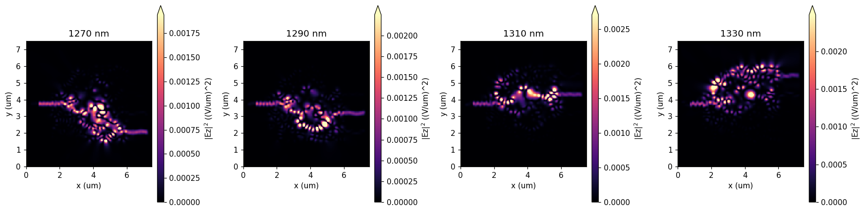
Compute modal power, total flux, and a field map at each channel center. A fresh ordinary simulation samples 151 frequencies. Additional incident-normalized spectra are reported separately; values are not clipped. The source has a finite spectral range, so inspect the input spectrum before interpreting far-band tails.
frequency_spacing=abs(np.diff(frequencies_design).mean())
freqs_measure=np.linspace(frequencies_design.min()-frequency_spacing,frequencies_design.max()+frequency_spacing,151)
mode_monitors=[m.updated_copy(freqs=freqs_measure) for m in final_simulation.monitors]
flux_monitors=[FluxMonitor(center=m.center,size=m.size,freqs=freqs_measure,name=f"flux_{i}") for i,m in enumerate(mode_monitors[:4])]
field_monitor=FieldMonitor(center=(3.75*um,3.75*um,0),size=(7.5*um,7.5*um,0),freqs=frequencies_design,fields=("Ez",),name="field")
verified=final_simulation.updated_copy(monitors=[*mode_monitors,*flux_monitors,field_monitor]).run(backend="jax",performance=False)
modal_power=np.stack([np.abs(verified.mode(f"mode_{i}").amps.sel(direction="+",mode_index=0).values).reshape(-1)**2 for i in range(4)])
incident_power=np.abs(verified.mode("input").amps.sel(direction="+",mode_index=0).values).reshape(-1)**2
flux_power=np.stack([np.asarray(verified[f"flux_{i}"].flux).reshape(-1) for i in range(4)])
wavelengths_nm=LIGHT_SPEED/freqs_measure/1e-9
fig,axes=plt.subplots(1,2,figsize=(13,4))
for ax,powers,title in [(axes[0],modal_power,"Fundamental-mode power"),(axes[1],flux_power,"Total flux")]:
    for i in range(4):
        ax.plot(wavelengths_nm,10*np.log10(np.maximum(powers[i],1e-15)),label=f"Port {i}: {wavelengths_design[i]/1e-9:.0f} nm")
        bounds=LIGHT_SPEED/channel_frequencies[i,[0,-1]]/1e-9
        ax.axvspan(min(bounds),max(bounds),alpha=.08)
    ax.set(xlabel="Wavelength (nm)",ylabel="Source-normalized power (dB)",title=title,ylim=(-45,3))
    ax.legend();ax.grid(alpha=.25)
fig.tight_layout();plt.show()
fig,axes=plt.subplots(1,4,figsize=(16,4))
for f,ax,w in zip(frequencies_design,axes,wavelengths_design):
    verified.plot_field("field",field_name="Ez",val="abs^2",frequency=f,ax=ax)
    ax.set_title(f"{w/1e-9:.0f} nm")
fig.tight_layout();plt.show()
Binary export and independent verification
Threshold the final pattern into ordinary polygons. Compare the same geometry at 50 and 30 nm, and double the duration on the finer mesh. Report each channel's intended transmission, unwanted-port power, and isolation using independently measured incident power. This sensitivity study is not a proof of mesh convergence or fabrication readiness.
binary=result.export_design()
verification_rows=[]
for resolution,duration in [(50e-9,6e-12),(30e-9,6e-12),(30e-9,12e-12)]:
    sim=design.simulation.updated_copy(design=binary,resolution=resolution,run_time=duration)
    data=sim.run(backend="jax",performance=False)
    output=np.asarray(channel_powers({f"mode_{i}":data.mode(f"mode_{i}") for i in range(4)}))
    input_samples=np.abs(data.mode("input").amps.sel(direction="+",mode_index=0).values.reshape(4,5))**2
    normalized=np.stack([np.abs(data.mode(f"mode_{i}").amps.sel(direction="+",mode_index=0).values.reshape(4,5))**2/input_samples for i in range(4)]).mean(axis=-1)
    desired=np.diag(normalized)
    unwanted=normalized.copy();np.fill_diagonal(unwanted,0)
    isolation=10*np.log10(desired/np.maximum(unwanted.max(axis=0),1e-15))
    row=dict(mesh_nm=resolution/1e-9,run_time_ps=duration/1e-12,desired=desired.tolist(),max_unwanted=unwanted.max(axis=0).tolist(),isolation_db=isolation.tolist())
    verification_rows.append(row)
    print(row,flush=True)
fig,ax=sim.plot(figsize=(7,6));ax.set_title("Exported binary WDM");plt.show()
metrics=dict(gradient_errors=gradient_errors,profile=profile,gradient_backend=design.gradient_backend,adjoint_source_grouping=design.adjoint_source_grouping,optimization_seconds=optimization_seconds,verification=verification_rows)
(artifacts/"metrics.json").write_text(json.dumps(metrics,indent=2))
np.savez_compressed(artifacts/"spectra.npz",frequencies=freqs_measure,modal_power=modal_power,incident_power=incident_power,flux_power=flux_power)
display(Markdown("**Finer-grid binary verification:** desired channel transmissions = "+", ".join(f"{v:.1%}" for v in verification_rows[-1]["desired"])+". See the full per-channel leakage and mesh/duration comparisons above."))
{'mesh_nm': 49.99999999999999, 'run_time_ps': 6.0, 'desired': [0.644935309269874, 0.7042425967562262, 0.8264931651368135, 0.24786979789317024], 'max_unwanted': [0.024510473800356026, 0.06990687032724444, 0.03852908658691345, 0.03588666139986678], 'isolation_db': [14.201644481051957, 10.032024306672337, 13.314505531602636, 8.392905556375966]}
{'mesh_nm': 29.999999999999996, 'run_time_ps': 6.0, 'desired': [0.4136358019644186, 0.45207343479825424, 0.42472186744168877, 0.15072356594966196], 'max_unwanted': [0.23832980108052843, 0.1967322957967204, 0.17362311868178026, 0.032556764982231215], 'isolation_db': [2.394397712640707, 3.613333272809944, 3.8849706895743106, 6.655399159960336]}
{'mesh_nm': 29.999999999999996, 'run_time_ps': 12.0, 'desired': [0.41363563550157706, 0.4520735678007773, 0.42472201021875194, 0.15072360391745937], 'max_unwanted': [0.23832985323051722, 0.19673226441147787, 0.17362315193581682, 0.03255677156014033], 'isolation_db': [2.394395014574828, 3.6133352433702663, 3.8849713177204177, 6.655399376496102]}
What this adds to BeamZ
Reusable projection/penalty/objective schedules, schedule-aware checkpoint continuation and export, optional broadband source-basis adjoints, and a four-channel WDM example. Both gradient backends share the same beamz.optimization workflow. General shape derivatives, dispersive material gradients, and multiple independent input excitations remain separate features.
Related device literature: Cheung et al., Inverse-designed CWDM demultiplexer operated in O-band, OFC 2024.
Export the binary layout to GDS
Install the optional layout dependency with pip install "beamz[gds]". Export the final projected density at threshold 0.5 together with the fixed input/output waveguides. The low-index background and the design-region clearing polygons are excluded, leaving only the core mask on layer 0/0. Coordinates are converted from metres to GDS micrometres by export_gds; polygon holes are preserved.
Files go to results/topology_examples/gds by default. Set BEAMZ_GDS_DIR to choose another destination. GDS stores the planar mask, not a layer thickness or a substrate. These layouts are example simulation results, not fabrication-qualified masks.
This is a 2D model; any thickness used for a 3D rendering is a visualization choice.
import os
from uuid import uuid4
from beamz.design import export_gds

# Unique cell names allow re-running this cell in the same gdsfactory session.

gds_root = next(p for p in [Path.cwd(), *Path.cwd().parents] if (p / "pyproject.toml").exists())
gds_dir = Path(os.environ.get("BEAMZ_GDS_DIR", gds_root / "results/topology_examples/gds")).expanduser()
gds_dir.mkdir(parents=True, exist_ok=True)

binary_layout = result.export_design(threshold=0.5)
# Clearing polygons represent cladding, not material to pattern.
core_layout = Design(
    width=binary_layout.width, height=binary_layout.height, depth=binary_layout.depth,
    background=binary_layout.background,
    structures=[s for s in binary_layout.structures
                if s.material.permittivity > binary_layout.background.permittivity],
)
gds_path = export_gds(core_layout, gds_dir / "topology_wdm_4channel.gds",
                      cell_name=f"wdm_4channel_{uuid4().hex[:8]}")
print(f"GDS core mask (layer 0/0): {gds_path.resolve()}")