 BeamZ
Topology optimization of a 3D waveguide bend
Goal
Optimize a 3D waveguide bend using beamz.optimization. A 3 × 3 µm planar pattern, extruded through 200 nm, couples perpendicular 500 nm wide waveguides. The electromagnetic simulation is fully vectorial and three-dimensional.
The model uses relative permittivities 1 and 4 and a 1 µm target wavelength. BeamZ uses metre units, (y, x) parameters, its own mode solver/material sampling, and local JAX execution. This is an exploratory optimization workflow.
Computation choices
- 50 nm uniform mesh. Four cells resolve the thickness; this is an exploratory mesh.
- 400 fs training runs and a broader Gaussian pulse, with explicit forward and adjoint decay guards.
- Ten Adam updates, learning rate 0.1 and fixed projection strength 5, using the high-level API. These are workflow demonstration settings, not a fabrication target.
- Final plots and a separate 800 fs verification show the actual simulation results. The notebook also rerasterizes exported polygons at 40 nm for a mesh-sensitivity check.
Both gradient backends are selectable. Full autodiff is checked on a smaller 100 nm version to keep its time-history memory manageable.
from pathlib import Path
import gc, json, time
import numpy as np
import jax
import jax.numpy as jnp
import matplotlib.pyplot as plt
from IPython.display import Markdown, display
from beamz import (LIGHT_SPEED, PML, Design, FieldMonitor, GaussianPulse, Material,
                   ModeMonitor, ModeSource, ModeSpec, Rectangle, Simulation)
import beamz.optimization as bi

root = Path.cwd()
while not (root / "pyproject.toml").exists() and root != root.parent:
    root = root.parent
artifacts = root / "results/topology_examples/topology_bend_3d"
artifacts.mkdir(parents=True, exist_ok=True)
um = 1e-6
frequency = LIGHT_SPEED / um
dx = 50e-9
run_time = 400e-15
num_steps = 10
plt.rcParams.update({"figure.dpi": 110, "font.size": 10})
print("Backend:", jax.default_backend(), "| mesh:", dx/1e-9, "nm")
Backend: cpu | mesh: 49.99999999999999 nm
Setup
Define the reference geometry and native inverse-design objects
The parameter grid is two-dimensional; InverseDesign broadcasts it through the finite z extent. Filters and penalties act on that planar pattern. No optimizer symmetry projection is imposed; the reference does not use one.
def make_bend(resolution=dx, duration=run_time, gradient_backend="adjoint"):
    geometry = Design(width=5*um, height=5*um, depth=2.2*um, material=Material(1))
    geometry += Rectangle(position=(0, 2.25*um, um), width=um, height=.5*um,
                          depth=.2*um, material=Material(4))
    geometry += Rectangle(position=(2.25*um, 0, um), width=.5*um, height=um,
                          depth=.2*um, material=Material(4))
    modes = ModeSpec(num_modes=1, polarization="te")
    source = ModeSource(center=(um/3, 2.5*um, 1.1*um), size=(0, 1.5*um, 2.2*um),
                        direction="+", mode_spec=modes,
                        source_time=GaussianPulse(freq0=frequency, fwidth=frequency/20,
                                                  offset=5/(2*np.pi)))
    output = ModeMonitor(center=(2.5*um, um/3, 1.1*um), size=(1.5*um, 0, 2.2*um),
                         freqs=[frequency], mode_spec=modes, name="mode")
    simulation = Simulation(design=geometry, resolution=resolution, run_time=duration,
                            sources=[source], monitors=[output],
                            boundaries=[PML(thickness=.3*um, formulation="cpml")])
    region = bi.TopologyDesignRegion(center=(2.5*um, 2.5*um, 1.1*um),
        size=(3*um, 3*um, .2*um), pixel_size=resolution, eps_bounds=(1, 4),
        transformations=[bi.FilterProject(radius=.15*um, beta=5)],
        penalties=[bi.ErosionDilationPenalty(length_scale=.15*um, weight=1)])
    return bi.InverseDesign(simulation=simulation, design_region=region,
                           gradient_backend=gradient_backend, checkpoint_interval=128)

def post_process(data):
    amplitude = data["mode"].amps.sel(direction="-", mode_index=0).values
    return jnp.sum(jnp.abs(amplitude)**2)

design = make_bend()
params0 = design.design_region.initial_parameters
initial_simulation = design.initial_simulation
print("Parameters:", params0.shape, "| count:", params0.size)
print("Material grid:", initial_simulation._material_grid().shape)
Parameters: (60, 60) | count: 3600 Material grid: (44, 100, 100)
Inspect the geometry and thickness
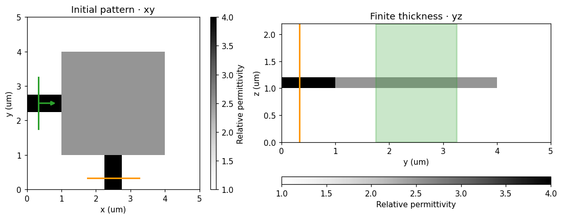
These are native Simulation.plot() and Simulation.plot_eps() views, including the x-normal cross-section used in the reference.
fig, ax = initial_simulation.plot(z=1.11*um, figsize=(6,5))
ax[0].set_title("3D bend: geometry at z = 1.11 µm")
plt.show()
fig, axes = plt.subplots(1,2,figsize=(11,4))
initial_simulation.plot_eps(z=1.11*um, ax=axes[0], vmin=1, vmax=4, title="Initial pattern · xy")
initial_simulation.plot_eps(x=2.51*um, ax=axes[1], vmin=1, vmax=4, title="Finite thickness · yz")
plt.show()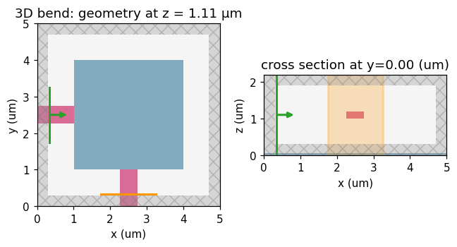
Checks
Compare full autodiff, spectral adjoint, and finite differences
Use the same reference geometry at 100 nm. This validates the vector derivative on an affordable fixture; it does not establish mesh convergence. A deterministic perturbation makes the comparison exercise nonuniform materials.
check_ad = make_bend(resolution=100e-9, gradient_backend="autodiff")
check_adj = check_ad.updated_copy(gradient_backend="adjoint")
check_params = check_ad.design_region.initial_parameters + np.random.default_rng(7).uniform(
    -.02, .02, check_ad.design_region.params_shape)
fun_ad = check_ad.make_objective_fn(post_process)
va, ga = jax.value_and_grad(fun_ad)(check_params)
vb, gb = jax.value_and_grad(check_adj.make_objective_fn(post_process))(check_params)
gradient_error = float(np.linalg.norm(ga-gb)/np.linalg.norm(ga))
direction = np.asarray(ga)/np.linalg.norm(ga)
h = .003
finite_difference = float((fun_ad(check_params+h*direction)-fun_ad(check_params-h*direction))/(2*h))
ad_directional = float(np.sum(ga*direction))
print(f"Adjoint/autodiff relative gradient difference: {100*gradient_error:.5f}%")
print(f"Directional derivative: autodiff={ad_directional:.7g}, finite difference={finite_difference:.7g}")
assert gradient_error < 3e-3
np.testing.assert_allclose(finite_difference, ad_directional, rtol=.01, atol=1e-7)
check_diagnostics = check_adj.gradient_diagnostics
print(check_diagnostics)
del check_ad, check_adj, fun_ad, ga, gb
jax.clear_caches(); gc.collect()
Adjoint/autodiff relative gradient difference: 0.00025%
Directional derivative: autodiff=0.02901014, finite difference=0.02900759
{'terminal_field_ratio': 2.8914112704114814e-07, 'decay_tolerance': 0.0001, 'adjoint_solves': 1, 'source_grouping': 'frequency', 'adjoint_terminal_field_ratios': (7.576031748612877e-07,), 'adjoint_timesteps': (2099,), 'stored_design_dft_values': 7502}
687Steps
Initial fields
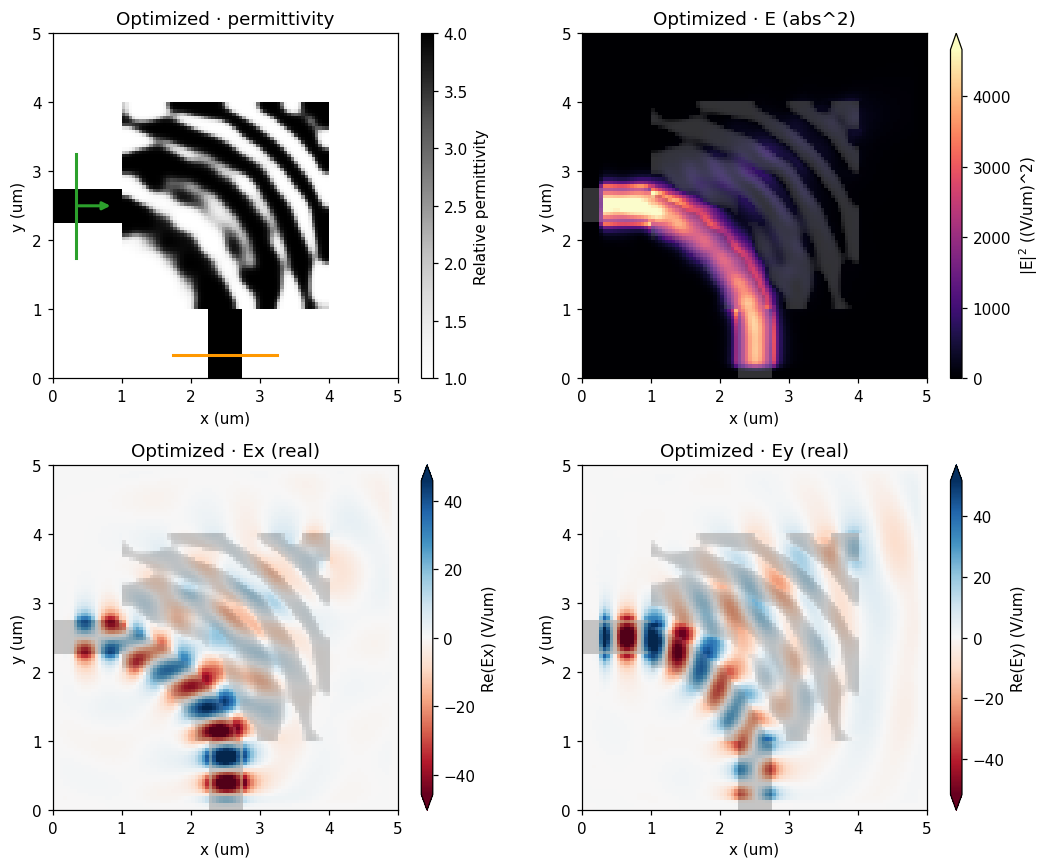
As in the reference, show permittivity, electric-field squared magnitude, and the real Ex/Ey components. All spatial plots use BeamZ utilities.
field_monitor = FieldMonitor(center=(2.5*um,2.5*um,1.1*um), size=(5*um,5*um,0),
                             freqs=[frequency], fields=("Ex","Ey","Ez"), name="field")
def field_run(simulation):
    return simulation.updated_copy(monitors=[*simulation.monitors,field_monitor]).run(
        backend="jax", performance=False)

def plot_reference_fields(simulation, data, title):
    fig, axes = plt.subplots(2,2,figsize=(11,8))
    simulation.plot_eps(z=1.11*um, ax=axes[0,0], vmin=1, vmax=4, title=title+" · permittivity")
    for axis, component, value in [(axes[0,1],"E","abs^2"),(axes[1,0],"Ex","real"),(axes[1,1],"Ey","real")]:
        data.plot_field("field", field_name=component, val=value, frequency=frequency, ax=axis)
        axis.set_title(f"{title} · {component} ({value})")
    fig.tight_layout()
    return fig

initial_fields = field_run(initial_simulation)
initial_power = float(np.sum(abs(initial_fields.mode("mode").amps.sel(direction="-",mode_index=0).values)**2))
plot_reference_fields(initial_simulation, initial_fields, "Initial")
plt.show()
print(f"Initial source-normalized target-mode power: {initial_power:.6f}")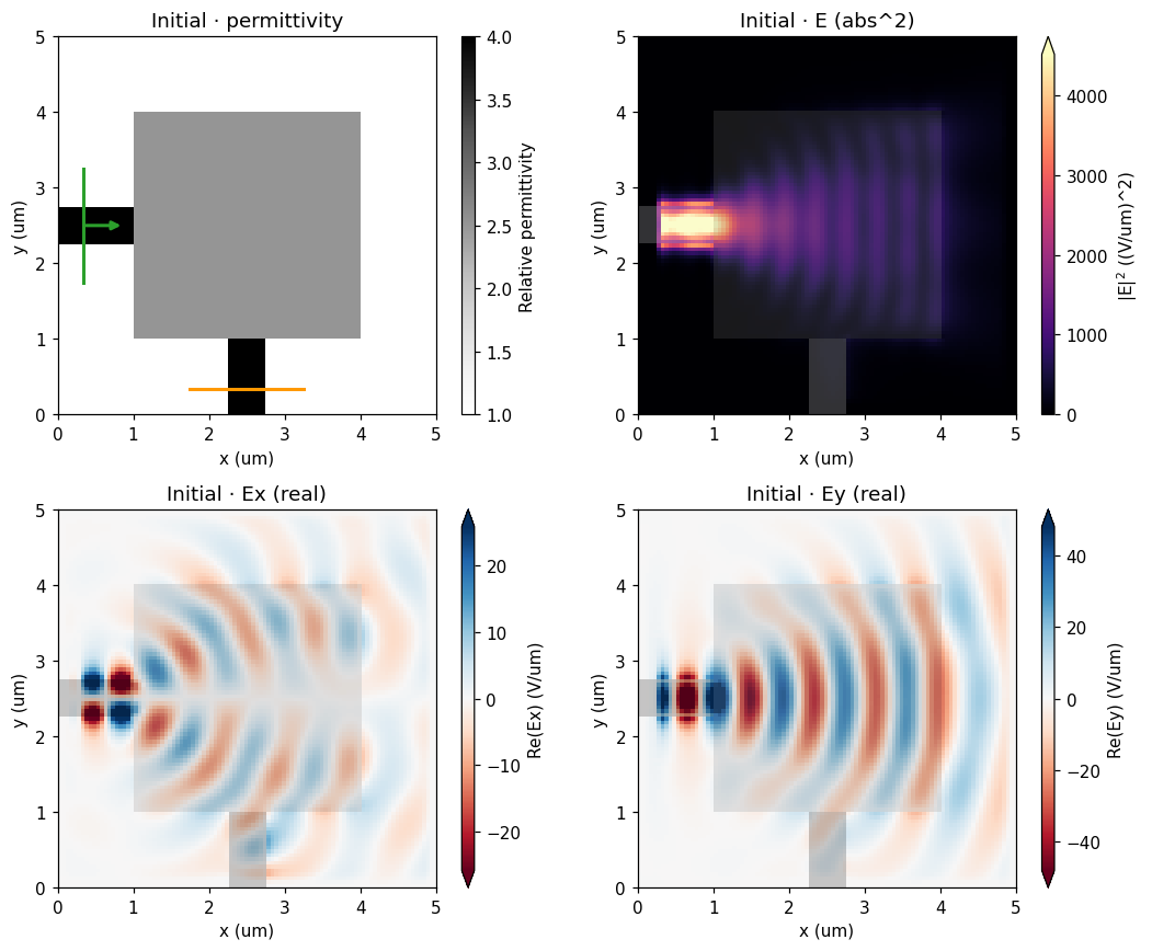
Initial source-normalized target-mode power: 0.004988
Optimize with the high-level workflow
Switch gradient_backend in make_bend to use full autodiff. The spectral adjoint retains only design-region electric DFTs, independent of timestep count. Every iteration checks forward and adjoint decay; an unconverged pulse raises an error.
optimizer = bi.AdamOptimizer(design=design, learning_rate=.1, objective_id="3d-bend-target-mode-power-v1")
started = time.perf_counter()
def progress(result):
    print(f"Step {result.completed_steps:2d}: power={result.history[-1].post_process_val:.6f}, "
          f"penalty={result.history[-1].penalty:.6f}, elapsed={time.perf_counter()-started:.1f} s", flush=True)
result = optimizer.run(post_process, steps=num_steps,
    checkpoint=artifacts/"history.npz", checkpoint_every=5, callback=progress)
optimization_seconds = time.perf_counter()-started
restored = optimizer.load_result(artifacts/"history.npz", post_process)
np.testing.assert_array_equal(restored.params[-1], result.params[-1])
print("Checkpoint restored exactly.")
np.testing.assert_allclose(result.history[0].post_process_val, initial_power, rtol=5e-5, atol=1e-7)
print(design.gradient_diagnostics)
Step 1: power=0.004988, penalty=1.000000, elapsed=137.8 s
Step 2: power=0.226613, penalty=1.000000, elapsed=285.4 s
Step 3: power=0.358087, penalty=1.000000, elapsed=458.9 s
Step 4: power=0.484459, penalty=0.999881, elapsed=608.5 s
Step 5: power=0.569794, penalty=0.977240, elapsed=731.7 s
Step 6: power=0.625841, penalty=0.928475, elapsed=887.9 s
Step 7: power=0.660765, penalty=0.881544, elapsed=1044.4 s
Step 8: power=0.692655, penalty=0.849435, elapsed=1210.3 s
Step 9: power=0.705467, penalty=0.809070, elapsed=1403.9 s
Step 10: power=0.724102, penalty=0.764608, elapsed=1624.2 s
Checkpoint restored exactly.
{'terminal_field_ratio': 2.8009787911287276e-07, 'decay_tolerance': 0.0001, 'adjoint_solves': 1, 'source_grouping': 'frequency', 'adjoint_terminal_field_ratios': (1.3787675925414078e-06,), 'adjoint_timesteps': (4197,), 'stored_design_dft_values': 51484}
Optimization history and final fields
History values are evaluated before each Adam update. Final performance below is evaluated after the last update. The penalized objective and optical power are reported separately.
fig, ax = plt.subplots(figsize=(7,4))
result.plot_optimization(ax=ax)
ax.set_title("3D bend optimization")
plt.show()
final_simulation = result.to_simulation()
final_fields = field_run(final_simulation)
final_power = float(np.sum(abs(final_fields.mode("mode").amps.sel(direction="-",mode_index=0).values)**2))
plot_reference_fields(final_simulation, final_fields, "Optimized")
plt.show()
assert final_power > initial_power
print(f"Target-mode power: {initial_power:.6f} → {final_power:.6f}")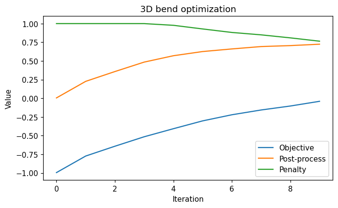
Target-mode power: 0.004988 → 0.734932
Transmission spectrum and longer-run verification
The reference plots transmission versus wavelength. Here an ordinary 800 fs FDTD run evaluates the final continuous design over 0.9–1.1 µm. This plot is source-normalized modal power; it is not normalized by a separately measured incident port. No values are clipped to the physical interval.
wavelengths = np.linspace(.9,1.1,41)*um
spectral_monitor = final_simulation.monitors[0].updated_copy(freqs=LIGHT_SPEED/wavelengths)
verification = final_simulation.updated_copy(run_time=800e-15,monitors=[spectral_monitor]).run(
    backend="jax", performance=False)
power_spectrum = np.abs(verification.mode("mode").amps.sel(direction="-",mode_index=0).values)**2
power_spectrum = np.asarray(power_spectrum).reshape(-1)
long_power = float(power_spectrum[len(wavelengths)//2])
fig, ax = plt.subplots(figsize=(7,4))
ax.plot(wavelengths/um,10*np.log10(np.maximum(power_spectrum,1e-15)),color="red")
ax.set(xlabel="Wavelength (µm)",ylabel="Target-mode power (dB)",title="Optimized 3D bend · 800 fs verification")
ax.grid(alpha=.25)
plt.show()
print(f"400 → 800 fs: {final_power:.6f} → {long_power:.6f}; change={100*(long_power-final_power):.4f} percentage points")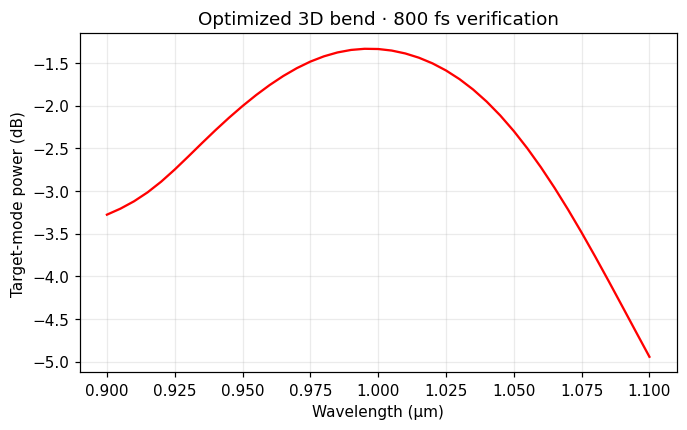
400 → 800 fs: 0.734932 → 0.734932; change=0.0000 percentage points
Export and independently rerasterize the binary geometry
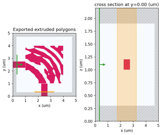
export_design() creates ordinary polygons with the correct extrusion height. Compare the same exported geometry at 50 and 40 nm; thresholding and mesh changes are distinct effects. Five cells resolve the thickness at 40 nm, so a smaller change is not proof of full mesh convergence.
binary_geometry = design.export_design(result.params[-1])
binary_powers = {}
for resolution in (50e-9,40e-9):
    binary_simulation = design.simulation.updated_copy(design=binary_geometry,
        resolution=resolution,run_time=800e-15)
    binary_data = binary_simulation.run(backend="jax",performance=False)
    binary_powers[float(resolution)] = float(np.sum(abs(binary_data.mode("mode").amps.sel(
        direction="-",mode_index=0).values)**2))
    print(f"Binary export at {resolution/1e-9:.0f} nm: {binary_powers[float(resolution)]:.6f}")
fig, ax = binary_simulation.plot(z=1.11*um,figsize=(6,5))
ax[0].set_title("Exported extruded polygons")
plt.show()
Binary export at 50 nm: 0.714983 Binary export at 40 nm: 0.745034
Results
The summary is calculated from this execution. The notebook demonstrates the optimization workflow; it does not establish mesh convergence or fabrication readiness.
metrics = dict(initial_power=initial_power,final_power=final_power,long_run_power=long_power,
               gradient_relative_error=gradient_error,optimization_seconds=optimization_seconds,
               binary_power_50nm=binary_powers[50e-9],binary_power_40nm=binary_powers[40e-9],
               mesh_nm=dx/1e-9,num_steps=num_steps,run_time_fs=run_time/1e-15)
(artifacts/"metrics.json").write_text(json.dumps(metrics,indent=2)+"\n")
np.savez_compressed(artifacts/"spectra.npz",wavelengths=wavelengths,power=power_spectrum)
display(Markdown(f"**Full 3D result:** source-normalized target-mode power improved from "
    f"**{initial_power:.4f} to {final_power:.4f}** after {num_steps} updates at {dx/1e-9:g} nm. "
    f"The 800 fs value is **{long_power:.4f}**. On the coarse gradient fixture, the backends "
    f"differ by **{100*gradient_error:.5f}%**. The exported binary geometry gives "
    f"**{binary_powers[50e-9]:.4f} / {binary_powers[40e-9]:.4f}** at 50 / 40 nm."))
Next steps
The same API now supports extruded patterns in vector 3D with both gradient routes, native plots, checkpoint restoration, and polygon export. General volumetric filter/penalty workflows, shape derivatives, multiple independent excitations, and lossy/dispersive gradients remain separate milestones.
Export the binary layout to GDS
Install the optional layout dependency with pip install "beamz[gds]". Export the final projected density at threshold 0.5 together with the fixed input/output waveguides. The low-index background and the design-region clearing polygons are excluded, leaving only the core mask on layer 0/0. Coordinates are converted from metres to GDS micrometres by export_gds; polygon holes are preserved.
Files go to results/topology_examples/gds by default. Set BEAMZ_GDS_DIR to choose another destination. GDS stores the planar mask, not a layer thickness or a substrate. These layouts are example simulation results, not fabrication-qualified masks.
The modeled core is 200 nm thick; retain that thickness when extruding this mask for 3D visualization.
import os
from uuid import uuid4
from beamz.design import export_gds

# Unique cell names allow re-running this cell in the same gdsfactory session.

gds_root = next(p for p in [Path.cwd(), *Path.cwd().parents] if (p / "pyproject.toml").exists())
gds_dir = Path(os.environ.get("BEAMZ_GDS_DIR", gds_root / "results/topology_examples/gds")).expanduser()
gds_dir.mkdir(parents=True, exist_ok=True)

binary_layout = result.export_design(threshold=0.5)
# Clearing polygons represent cladding, not material to pattern.
core_layout = Design(
    width=binary_layout.width, height=binary_layout.height, depth=binary_layout.depth,
    background=binary_layout.background,
    structures=[s for s in binary_layout.structures
                if s.material.permittivity > binary_layout.background.permittivity],
)
gds_path = export_gds(core_layout, gds_dir / "topology_bend_3d.gds",
                      cell_name=f"topology_bend_3d_{uuid4().hex[:8]}")
print(f"GDS core mask (layer 0/0): {gds_path.resolve()}")