Volumetric inverse design of a polarization-insensitive grating coupler

Optimize a 10 × 10 × 5 µm polymer volume on glass with BeamZ to couple a 5.2 µm Gaussian beam tilted by 10° into the TE₀₀ and TM₀₀ modes of a 2 × 2 µm waveguide, at 1.55 µm.

The objective is the mean coupling efficiency, $J=(\eta_{x\rightarrow\mathrm{TM}_{00}}+\eta_{y\rightarrow\mathrm{TE}_{00}})/2$ . Density varies along all three dimensions; y-mirror symmetry ties mirrored voxels. The two forward/adjoint experiments share one density array. This local BeamZ workflow supports GPU execution.

Run: install this branch with uv pip install -e '.[dev]' 'jax[cuda12]' (omit CUDA on CPU), then select its Python kernel. The default reference profile uses the geometry above, 50 nm design pixels, 20 Adam updates at learning rate 0.5, 0.4 µm filter radius, and β = 1…20. Set BEAMZ_GRATING_PROFILE=smoke before launching Jupyter for a coarse, three-update execution check. Saved outputs identify the profile actually executed.

Simulation setup: the FDTD grid is uniform, with a 100 nm step in the reference profile; the density grid uses 50 nm pixels. We simulate the full y domain and enforce mirror symmetry on density. The beam propagates toward +x and −z. The source plane has a three-cell clearance from the design; its waist remains at that plane. The output monitor is at x = 6 µm, in the uniform waveguide before the absorber starts at x = 6.5 µm. The z domain is rounded outward for grid alignment. Mesh convergence and fabrication suitability require further validation.

Python [1]

import os
from pathlib import Path
import time

import jax
import jax.numpy as jnp
import matplotlib.pyplot as plt
from matplotlib.colors import Normalize, LightSource
from mpl_toolkits.mplot3d.art3d import Poly3DCollection
import numpy as np
import optax
from skimage.measure import marching_cubes

import beamz as bz
import beamz.optimization as opt

profile = os.environ.get("BEAMZ_GRATING_PROFILE", "reference")
if profile not in {"reference", "smoke"}:
    raise ValueError("BEAMZ_GRATING_PROFILE must be reference or smoke")
dx = (0.10 if profile == "reference" else 0.25) * bz.um
density_dx = (0.05 if profile == "reference" else 0.25) * bz.um
steps = 20 if profile == "reference" else 3
wavelength = 1.55 * bz.um
frequency = bz.LIGHT_SPEED / wavelength
run_time = 50 / (frequency / 10)
output_dir = Path("results/polarization_insensitive_grating") / profile
output_dir.mkdir(parents=True, exist_ok=True)
plt.rcParams.update({"figure.dpi": 120, "font.size": 11, "axes.spines.top": False,
                     "axes.spines.right": False, "savefig.bbox": "tight"})
colors = ("#2864b4", "#ca781c")
print(f"Profile: {profile} | devices: {jax.devices()} | FDTD: {dx/bz.um:g} µm | "
      f"density: {density_dx/bz.um:g} µm | {steps} updates | pulse run: {run_time*1e12:.3f} ps")

Profile: reference | devices: [CudaDevice(id=0)] | FDTD: 0.1 µm | density: 0.05 µm | 20 updates | pulse run: 2.585 ps

Geometry and the two illumination experiments

Polymer has $n = 1.53$ , glass $n = 1.444$ , and the background is air. The glass top is at z = −2.5 µm, flush with the design bottom; the output guide occupies z = −2.5…−0.5 µm. Explicit TE and TM mode bases select the two target channels in the full simulation domain. The conic filter is spherical in 3D; projection sharpness increases during optimization. Filtering encourages smooth features but does not guarantee a fabrication limit or connectivity.

Mode-label convention: for the output guide propagating along x, TE₀₀ is Ey-dominated and TM₀₀ is Ez-dominated. The two experiments pair x-polarized illumination with TM₀₀ and y-polarized illumination with TE₀₀, using explicit polarization-aware mode selection.

Python [2]

rho_size = np.array([10, 10, 5]) * bz.um
size = np.array([15 * bz.um, 15 * bz.um,
                 2 * np.ceil((4 + 5 + 1.55) * bz.um / (2 * dx)) * dx])
polymer, glass = bz.Material(1.53**2), bz.Material(1.444**2)
geometry = bz.Design(background=bz.Material(1))
# Public geometry coordinates are centered in the simulation domain.
geometry += bz.Box(center=(0, 0, (-size[2]/2 - 2.5*bz.um)/2),
                   size=(size[0], size[1], size[2]/2 - 2.5*bz.um), material=glass)
geometry += bz.Box(center=(7.5*bz.um, 0, -1.5*bz.um),
                   size=(5*bz.um, 2*bz.um, 2*bz.um), material=polymer)


def mirror_y(density, pixel_size):
    return (density + jnp.flip(density, axis=1)) / 2


region = opt.TopologyDesignRegion(
    center=(0, 0, 0), size=tuple(rho_size), pixel_size=density_dx,
    eps_bounds=(1, 1.53**2), parameterization="volumetric",
    transformations=[mirror_y, opt.FilterProject(radius=0.4*bz.um), mirror_y],
    initialization_spec=opt.RandomInitializationSpec(seed=42),
)
pulse = bz.GaussianPulse(freq0=frequency, fwidth=frequency/10)
source_z = (2.5*bz.um + 3*dx)
beam = bz.GaussianBeamSource(
    center=(0, 0, source_z), size=(13*bz.um, 13*bz.um),
    source_time=pulse, direction="-z", angle_theta=np.deg2rad(10),  # Propagation toward +x and −z.
    waist_radius=2.6*bz.um, power=1,
)


def make_experiment(pol_angle, mode_polarization):
    output = bz.ModeMonitor(
        center=(6*bz.um, 0, -1.5*bz.um), size=(0, 6*bz.um, 6*bz.um),
        freqs=[frequency], name="output",
        mode_spec=bz.ModeSpec(num_modes=1, polarization=mode_polarization),
    )
    simulation = bz.Simulation(
        design=geometry, domain=tuple(size), resolution=dx, run_time=run_time,
        sources=[beam.updated_copy(pol_angle=pol_angle)], monitors=[output],
        boundaries=[bz.PML(thickness=1*bz.um, formulation="cpml")],
    )
    return opt.InverseDesign(simulation=simulation, design_region=region,
                             gradient_backend="adjoint")


experiments = [make_experiment(0, "tm"), make_experiment(np.pi/2, "te")]
params = jnp.asarray(region.initial_parameters)
print(f"Density shape (z, y, x): {params.shape}; {params.size:,} parameters")

Density shape (z, y, x): (100, 200, 200); 4,000,000 parameters

Inspect a real volume

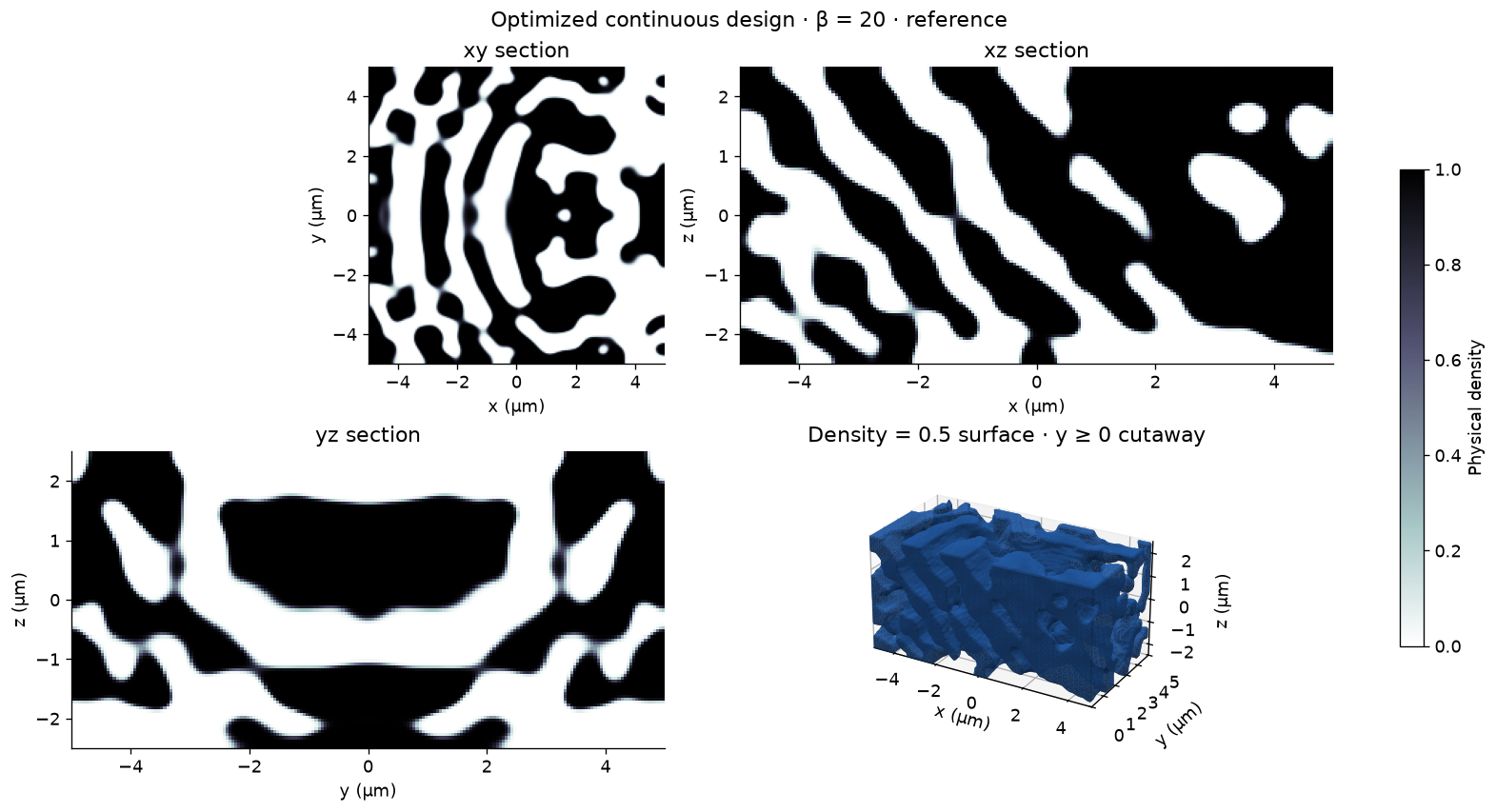
The middle xy, xz, and yz slices reveal variation along z. The surface panel renders the density = 0.5 boundary with a y ≥ 0 cutaway to expose the interior; it is a visualization of the continuous density, not a verified printable solid. Rendering may sample every second voxel on the fine grid, without changing the simulation.

Python [3]

def show_density(parameters, beta, title):
    density = np.asarray(region.material_density(parameters, beta=beta))
    fig = plt.figure(figsize=(13, 7), layout="constrained")
    axes = [fig.add_subplot(2, 2, i) for i in (1, 2, 3)]
    nz, ny, nx = density.shape
    slices = [density[nz//2], density[:, ny//2], density[:, :, nx//2]]
    extents = [(-5, 5, -5, 5), (-5, 5, -2.5, 2.5), (-5, 5, -2.5, 2.5)]
    for ax, values, extent, labels in zip(axes, slices, extents, [("x", "y"), ("x", "z"), ("y", "z")]):
        image = ax.imshow(values, origin="lower", extent=extent, vmin=0, vmax=1, cmap="bone_r")
        ax.set(xlabel=f"{labels[0]} (µm)", ylabel=f"{labels[1]} (µm)", title=f"{labels[0]}{labels[1]} section")
    fig.colorbar(image, ax=axes, shrink=0.7, label="Physical density")
    ax = fig.add_subplot(2, 2, 4, projection="3d")
    stride = 2 if density.shape[-1] > 100 else 1
    cutaway = density.copy()
    cutaway[:, :ny//2, :] = 0  # Rendering only: expose the symmetry-plane interior.
    sampled = np.pad(cutaway[::stride, ::stride, ::stride], 1)
    if sampled.max() > 0.5:
        verts, faces, _, _ = marching_cubes(sampled, level=0.5, step_size=1)
        verts = ((verts - 1)*stride + 0.5) * density_dx / bz.um
        verts -= np.array([2.5, 5, 5])
        surface = Poly3DCollection(verts[faces][:, :, ::-1], facecolors=colors[0],
                                   edgecolor="none", shade=True, lightsource=LightSource(315, 45),
                                   rasterized=True)
        ax.add_collection3d(surface)
    ax.set(xlim=(-5, 5), ylim=(0, 5), zlim=(-2.5, 2.5), xlabel="x (µm)",
           ylabel="y (µm)", zlabel="z (µm)", title="Density = 0.5 surface · y ≥ 0 cutaway")
    ax.set_box_aspect((2, 1, 1))
    ax.view_init(elev=25, azim=-60)
    fig.suptitle(f"{title} · β = {beta:g} · {profile}")
    return fig


show_density(params, beta=1, title="Initial design");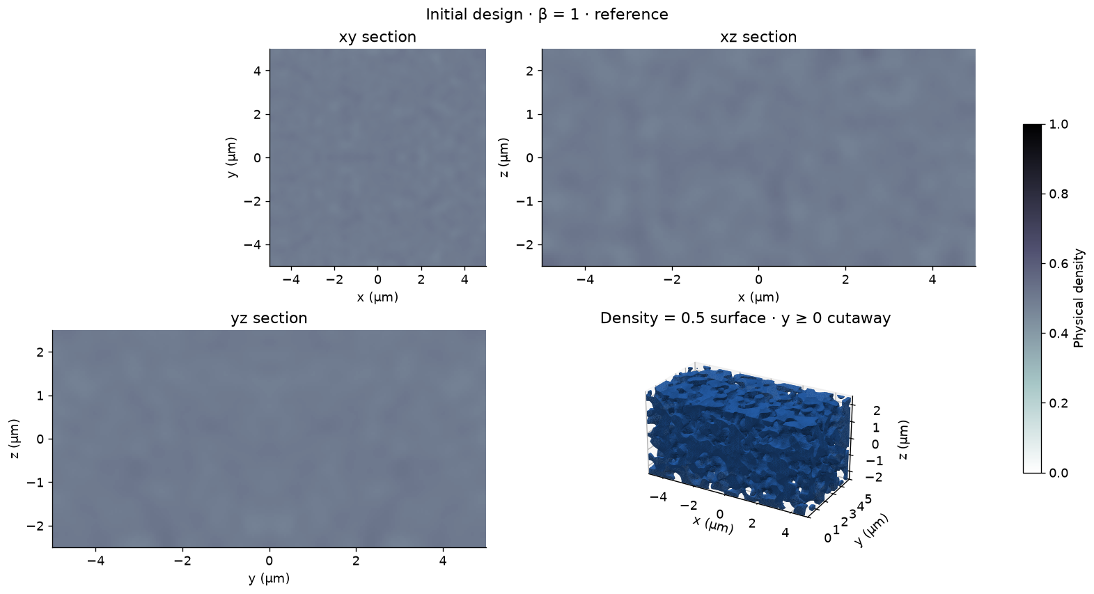

Shared-density objective and gradient check

Amplitudes are normalized by the Gaussian pulse spectrum and projected into power-normalized output modes. Divide $∣ a ∣^{2}$ by the fixed incident power (1 W here) to obtain coupling efficiency. The adjoint retains design-region electric DFTs rather than the entire time history and checks that both forward and adjoint fields decay.

The directional finite-difference check below probes the combined two-polarization objective, including symmetry, filtering, projection, resampling, and the Yee material map. A second run-time check near the end tests whether truncated transients materially change the answer.

Python [4]

def coupling_efficiencies(parameters, beta):
    return jnp.stack([
        opt.ModePower("output")(experiment.to_simulation_data(parameters, beta=beta))
        for experiment in experiments
    ])


def objective(parameters, beta):
    efficiencies = coupling_efficiencies(parameters, beta)
    return jnp.mean(efficiencies), efficiencies


evaluate = jax.value_and_grad(objective, has_aux=True)
(initial_value, initial_ce) = objective(params, 1.0)
check_params = 0.1 + 0.8*params  # Keep finite-difference probes inside [0, 1].
(_, _), gradient = evaluate(check_params, 1.0)
direction = gradient / jnp.linalg.norm(gradient)
h = 0.01
finite_difference = (objective(check_params+h*direction, 1.0)[0] - objective(check_params-h*direction, 1.0)[0]) / (2*h)
adjoint_derivative = jnp.vdot(gradient, direction).real
relative_error = float(abs(finite_difference-adjoint_derivative) / abs(adjoint_derivative))
assert np.isfinite(gradient).all() and np.linalg.norm(gradient) > 0
assert relative_error < 0.02, f"Gradient check error: {relative_error:.4%}"
print(f"Initial CE: x→TM {float(initial_ce[0]):.4%}, y→TE {float(initial_ce[1]):.4%}")
print(f"Directional derivative: adjoint {float(adjoint_derivative):.6g}, "
      f"finite difference {float(finite_difference):.6g}; relative error {relative_error:.4%}")

Initial CE: x→TM 0.0001%, y→TE 0.0003%
Directional derivative: adjoint 6.79382e-06, finite difference 6.79378e-06; relative error 0.0005%

Twenty Adam updates with projection continuation

The reference learning rate is 0.5 and β increases by one each update. The history records pre-update efficiencies at that iteration's β; the final density is evaluated separately at the final β. Each checkpoint is a portable numerical snapshot (density, history, and settings), not a serialized Python object. This compact loop combines both simulations explicitly.

Python [5]

optimizer = optax.adam(learning_rate=0.5)
optimizer_state = optimizer.init(params)
initial_params = np.asarray(params).copy()
history = []
start = time.perf_counter()
for step in range(steps):
    beta = float(step + 1)
    (score, efficiencies), gradient = evaluate(params, beta)
    if not np.isfinite(gradient).all():
        raise FloatingPointError("Nonfinite design gradient")
    updates, optimizer_state = optimizer.update(-gradient, optimizer_state, params)
    params = jnp.clip(optax.apply_updates(params, updates), 0, 1)
    history.append([step, beta, *np.asarray(efficiencies)])
    np.savez_compressed(output_dir / "design.npz", density=np.asarray(params),
                        initial_density=initial_params, history=np.array(history),
                        profile=profile, fdtd_dx=dx, density_dx=density_dx, beta=beta)
    print(f"{step+1:2d}/{steps} · β={beta:g} · x→TM {float(efficiencies[0]):6.2%} · "
          f"y→TE {float(efficiencies[1]):6.2%} · mean {float(score):6.2%}")

final_beta = float(steps)
final_ce = np.asarray(coupling_efficiencies(params, final_beta))
history = np.asarray(history)
np.savez_compressed(output_dir / "design.npz", density=np.asarray(params),
                    initial_density=initial_params, history=history, final_ce=final_ce,
                    profile=profile, fdtd_dx=dx, density_dx=density_dx, beta=final_beta)
print(f"Final CE: x→TM {final_ce[0]:.2%}, y→TE {final_ce[1]:.2%}; "
      f"mean {final_ce.mean():.2%} | elapsed {(time.perf_counter()-start)/60:.1f} min")

 1/20 · β=1 · x→TM  0.00% · y→TE  0.00% · mean  0.00%
 2/20 · β=2 · x→TM  3.79% · y→TE 16.25% · mean 10.02%
 3/20 · β=3 · x→TM 19.88% · y→TE 22.24% · mean 21.06%
 4/20 · β=4 · x→TM 23.39% · y→TE 19.21% · mean 21.30%
 5/20 · β=5 · x→TM 33.29% · y→TE 32.76% · mean 33.02%
 6/20 · β=6 · x→TM 36.42% · y→TE 37.88% · mean 37.15%
 7/20 · β=7 · x→TM 42.22% · y→TE 46.51% · mean 44.37%
 8/20 · β=8 · x→TM 44.68% · y→TE 45.84% · mean 45.26%
 9/20 · β=9 · x→TM 51.80% · y→TE 55.40% · mean 53.60%
10/20 · β=10 · x→TM 53.79% · y→TE 55.80% · mean 54.79%
11/20 · β=11 · x→TM 59.68% · y→TE 60.34% · mean 60.01%
12/20 · β=12 · x→TM 60.22% · y→TE 61.97% · mean 61.10%
13/20 · β=13 · x→TM 62.06% · y→TE 65.36% · mean 63.71%
14/20 · β=14 · x→TM 64.02% · y→TE 66.82% · mean 65.42%
15/20 · β=15 · x→TM 65.38% · y→TE 66.35% · mean 65.87%
16/20 · β=16 · x→TM 66.61% · y→TE 68.46% · mean 67.53%
17/20 · β=17 · x→TM 66.86% · y→TE 69.67% · mean 68.27%
18/20 · β=18 · x→TM 67.70% · y→TE 70.29% · mean 69.00%
19/20 · β=19 · x→TM 69.03% · y→TE 70.46% · mean 69.74%
20/20 · β=20 · x→TM 69.51% · y→TE 70.84% · mean 70.17%
Final CE: x→TM 69.95%, y→TE 71.82%; mean 70.88% | elapsed 37.7 min

Python [6]

fig, axes = plt.subplots(1, 2, figsize=(12, 4), layout="constrained")
for index, label in enumerate(("x → TM₀₀", "y → TE₀₀")):
    axes[0].plot(history[:, 0], 100*history[:, index+2], "o-", color=colors[index], label=label)
    axes[0].scatter([steps], [100*final_ce[index]], marker="*", s=130, color=colors[index])
axes[0].plot(history[:, 0], 50*(history[:, 2]+history[:, 3]), "k--", label="Mean")
axes[0].set(xlabel="Adam update (0 = initial)", ylabel="Coupling efficiency (%)",
            title="Pre-update values; stars = final evaluation", ylim=(0, None))
axes[0].legend()
axes[1].bar([0, 1], 100*final_ce, color=colors, width=0.6)
axes[1].set(xticks=[0, 1], xticklabels=["x → TM₀₀", "y → TE₀₀"],
            ylabel="Coupling efficiency (%)", title="Final coupling at 1.55 µm", ylim=(0, 100))
for index, efficiency in enumerate(final_ce):
    axes[1].text(index, 100*efficiency+2, f"{efficiency:.2%}", ha="center")
fig.savefig(output_dir / "convergence.png")
show_density(params, final_beta, "Optimized continuous design").savefig(output_dir / "density.png");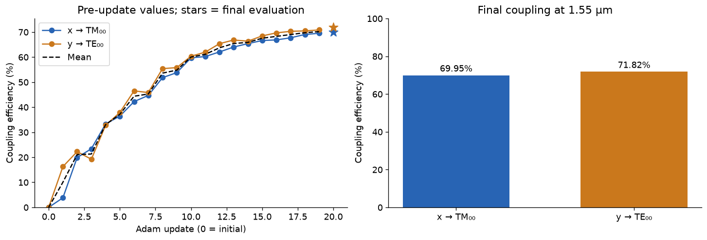

Broadband validation and electric-field sections

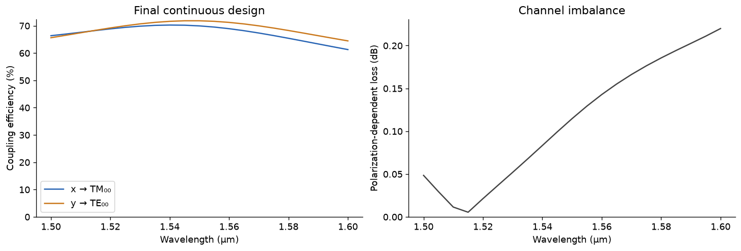
Run ordinary BeamZ simulations on the final continuous-density material grid. Record 21 wavelengths from 1.50 to 1.60 µm, and xy/xz electric-field sections at 1.55 µm. Coupling efficiencies use the same TE/TM definitions as optimization; the polarization-dependent loss is $10\log_{10}(\eta_{\max}/\eta_{\min})$ . Maximizing the mean does not itself force the channels to be equal, so we report both and their imbalance.

Python [7]

wavelengths = np.linspace(1.50, 1.60, 21) * bz.um
validation = []
for experiment in experiments:
    simulation = experiment.to_simulation(params, beta=final_beta)
    # Ordinary simulations keep normalized internal device coordinates.
    monitor = simulation.monitors[0]
    center = np.asarray(experiment.simulation.coordinate_offset)
    xy = bz.FieldMonitor(center=tuple(center + np.array([0, 0, -1.5])*bz.um),
                          size=(13*bz.um, 13*bz.um, 0), freqs=[frequency], name="xy",
                          fields=["Ex", "Ey", "Ez"])
    xz = bz.FieldMonitor(center=tuple(center), size=(13*bz.um, 0, 8*bz.um),
                          freqs=[frequency], name="xz", fields=["Ex", "Ey", "Ez"])
    simulation = simulation.updated_copy(monitors=[monitor.updated_copy(freqs=bz.LIGHT_SPEED/wavelengths), xy, xz])
    validation.append(simulation.run(backend="jax", performance=False))

spectra = np.stack([
    np.abs(result.mode("output").amps.sel(direction="+", mode_index=0).values)**2
    / result.launched_power(0) for result in validation
])
np.testing.assert_allclose(spectra[:, 10], final_ce, rtol=0.01, atol=1e-5)
fig, axes = plt.subplots(1, 2, figsize=(12, 4), layout="constrained")
for index, label in enumerate(("x → TM₀₀", "y → TE₀₀")):
    axes[0].plot(wavelengths/bz.um, 100*spectra[index], color=colors[index], label=label)
axes[0].set(xlabel="Wavelength (µm)", ylabel="Coupling efficiency (%)", ylim=(0, None), title="Final continuous design")
axes[0].legend()
pdl = 10*np.log10(np.maximum(spectra.max(axis=0), 1e-12)/np.maximum(spectra.min(axis=0), 1e-12))
axes[1].plot(wavelengths/bz.um, pdl, color="#444444")
axes[1].set(xlabel="Wavelength (µm)", ylabel="Polarization-dependent loss (dB)", ylim=(0, None), title="Channel imbalance")
fig.savefig(output_dir / "spectra.png")
np.savez_compressed(output_dir / "spectra.npz", wavelengths=wavelengths, coupling=spectra, pdl=pdl)
print(f"PDL at 1.55 µm: {pdl[10]:.3f} dB")

PDL at 1.55 µm: 0.115 dB

Python [8]

field_maps = [[np.sqrt(sum(abs(result[name].get_dft_component(component).reshape(-1))**2
                           for component in ("Ex", "Ey", "Ez")))
               for name in ("xy", "xz")] for result in validation]
# Frequency-domain acquisitions store flattened common-plane samples.
for pair, result in zip(field_maps, validation):
    for index, name in enumerate(("xy", "xz")):
        sampled = result[name].sample_region
        plane_axes = ("y", "x") if name == "xy" else ("z", "x")
        shape = tuple(sampled.intervals[axis].stop - sampled.intervals[axis].start for axis in plane_axes)
        pair[index] = pair[index].reshape(shape).squeeze()
fig, axes = plt.subplots(2, 2, figsize=(12, 8), layout="constrained")
norm = Normalize(0, max(float(field.max()) for pair in field_maps for field in pair))
for row, pair in enumerate(field_maps):
    for column, field in enumerate(pair):
        extent = (-6.5, 6.5, -6.5, 6.5) if column == 0 else (-6.5, 6.5, -4, 4)
        image = axes[row, column].imshow(field, origin="lower", extent=extent, cmap="inferno", norm=norm)
        axes[row, column].set(xlabel="x (µm)", ylabel=("y (µm)" if column == 0 else "z (µm)"),
                             title=f"{['x → TM₀₀', 'y → TE₀₀'][row]} · {['xy', 'xz'][column]} · |E| at 1.55 µm")
fig.colorbar(image, ax=axes.ravel().tolist(), shrink=0.8, label="Electric-field amplitude (V/m, pulse-normalized)")
fig.savefig(output_dir / "fields.png");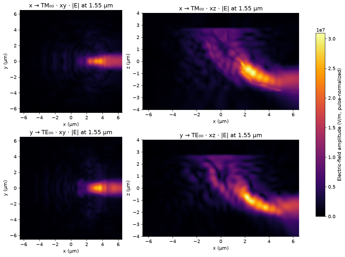

Check run duration and the thresholded geometry

A continuous-density optimum can use intermediate material values. Thresholding may change performance substantially. The binary check below runs the ordinary solver with a thresholded density through the same material map; it does not claim a manufacturable mesh or mesh convergence. Layered polygon export is available with experiments[0].export_design(params, beta=final_beta, mode="pixel_exact") for independent geometry rasterization.

Before reporting a final device, repeat with smaller FDTD steps (the reference density pixels are already 50 nm), longer run times, and the exported binary geometry. The coarse smoke profile is an execution check only.

Python [9]

long_ce, binary_ce = [], []
physical_density = np.asarray(region.material_density(params, beta=final_beta))
# Density is already mirrored; skip transforms so the thresholded values stay binary.
binary_region = region.updated_copy(transformations=[])
for experiment in experiments:
    continuous = experiment.to_simulation(params, beta=final_beta)
    longer = continuous.updated_copy(run_time=1.5*run_time).run(backend="jax", performance=False)
    long_ce.append(float(abs(longer.mode("output").amps.sel(direction="+", mode_index=0).values[0])**2 / longer.launched_power(0)))
    binary = experiment.updated_copy(design_region=binary_region).to_simulation((physical_density >= 0.5).astype(np.float32))
    result = binary.run(backend="jax", performance=False)
    binary_ce.append(float(abs(result.mode("output").amps.sel(direction="+", mode_index=0).values[0])**2 / result.launched_power(0)))
long_ce, binary_ce = np.array(long_ce), np.array(binary_ce)
relative_duration_change = np.max(abs(long_ce-final_ce) / np.maximum(final_ce, 1e-8))
print(f"50% longer run: x→TM {long_ce[0]:.2%}, y→TE {long_ce[1]:.2%}; "
      f"maximum relative change {relative_duration_change:.2%}")
print(f"Thresholded density: x→TM {binary_ce[0]:.2%}, y→TE {binary_ce[1]:.2%}")
assert relative_duration_change < 0.02, "Increase run_time and repeat before trusting the objective"
np.savez_compressed(output_dir / "checks.npz", continuous_ce=final_ce, longer_ce=long_ce,
                    binary_ce=binary_ce, gradient_relative_error=relative_error,
                    duration_relative_change=relative_duration_change)
print(f"Numerical arrays and figures saved to {output_dir.resolve()}")

50% longer run: x→TM 69.95%, y→TE 71.82%; maximum relative change 0.00%
Thresholded density: x→TM 70.14%, y→TE 71.75%
Numerical arrays and figures saved to /home/quentinwach/beamz/beamz-volumetric-grating/results/polarization_insensitive_grating/reference

The saved outputs above are BeamZ calculations for the printed profile. They demonstrate volumetric optimization and the two-channel workflow. Mesh convergence, minimum printable features, and structural integrity require additional validation before fabrication.