 BeamZ
CMOS RGB image sensor
Simulate a periodic 2 × 2 RGGB pixel array with silica microlenses, dispersive color filters, aluminum shielding and interconnects, a silicon-nitride antireflection coating, and an amorphous-silicon detector.
The workflow covers material spectra → geometry → broadband simulation → two vertical field profiles → detector-plane fields → optical efficiency. Materials are imported directly from beamz.material_library, which bundles the fitted coefficients, synthetic filter inputs, and license notices.
Simulation setup
Run with BeamZ and the notebook dependencies installed (pip install -e '.[dev]'). The full 3D calculation is intended for a GPU; the saved outputs can be viewed without running it. Select a Python kernel with CUDA-enabled JAX to use an NVIDIA GPU. All calculations use SI units.
from pathlib import Path
import hashlib
import pickle
import sys

import jax
import matplotlib.pyplot as plt
from matplotlib.patches import Circle, Patch, Rectangle
import numpy as np

ROOT = next(p for p in (Path.cwd(), *Path.cwd().parents) if (p / "beamz").is_dir())
sys.path.insert(0, str(ROOT))
import beamz as bz
from beamz import material_library

um = bz.um
plt.rcParams.update({"font.size": 11, "figure.dpi": 110})
print(f"BeamZ {bz.__version__}; JAX {jax.__version__}: {jax.devices()}")
BeamZ 0.5.2; JAX 0.9.0: [CudaDevice(id=0)]
Materials
Import the visible-band media directly from BeamZ. Silica and aluminum use CC0 optical data; silicon nitride and amorphous silicon use published Lorentz formulas. Synthetic RGB targets use n = 1.45, passband k = 0.01, stopband k = 0.46, and smooth 30 nm transitions. BeamZ's vector fitter weights real and imaginary permittivity by 0.1 and 1.9. The fitted indices disperse; achieved errors and tolerance flags are available in each material variant's fit metadata. Dashed curves show targets and solid curves show the fitted response.
materials = {
    "air": bz.Material(1.0),
    "silica": material_library["SiO2"]["Malitson1965"],
    "sin": material_library["SiN"]["Horiba2006"],
    "silicon": material_library["aSi"]["Horiba2006"],
    "metal": material_library["Al"]["Rakic1995"],
    **{name: material_library["CMOS_RGB"][name] for name in ("red", "green", "blue")},
}

fig, axes = plt.subplots(1, 3, figsize=(12, 3.5), layout="constrained")
for ax, channel in zip(axes, ("red", "green", "blue")):
    wavelength, n, k = material_library["CMOS_RGB"].variants[channel].nk_data.T
    fitted = np.sqrt(materials[channel].eps_model(bz.LIGHT_SPEED / wavelength))
    ax.plot(wavelength * 1e9, n, "k--", alpha=0.5, label="n target")
    ax.plot(wavelength * 1e9, k, "--", color=channel, alpha=0.5, label="k target")
    ax.plot(wavelength * 1e9, fitted.real, "k", label="n fit")
    ax.plot(wavelength * 1e9, fitted.imag, color=channel, label="k fit")
    ax.set(
        title=f"{channel.capitalize()} filter",
        xlabel="Wavelength (nm)",
        ylabel="n, k",
        xlim=(400, 700),
    )
axes[0].legend(fontsize=8)
plt.show()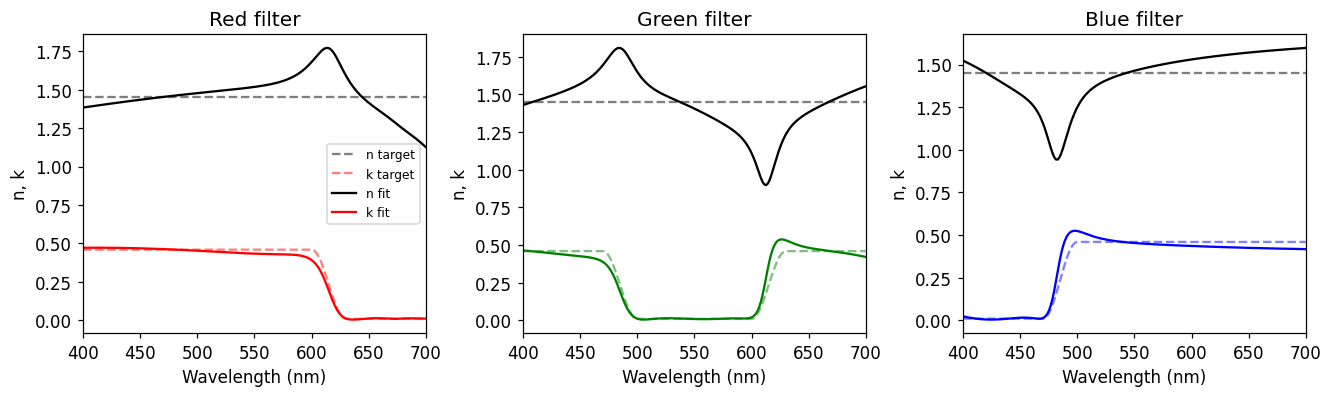
Dimensions and spectrum
The unit cell is 3 µm × 3 µm. The two green pixels are counted together. The silicon-nitride coating has a fixed thickness of 70.93385 nm. The source spans 400–700 nm, and the runtime is 510 fs.
Lx = Ly = 3.0 * um
d_absorber_space = 1.5 * um

pixel_width = Lx / 2
lens_radius = 1.0 * um
lens_height = (1 - np.cos(np.arcsin(pixel_width / (2 * lens_radius)))) * lens_radius

d_lens_to_filter = 0.2 * um
t_filter = 1.0 * um
d_filter_to_shield = 0.5 * um
t_shield = 0.10 * um
shield_hole_radius = 0.95 * pixel_width
d_shield_to_connect = 0.5 * um
t_connect = 0.10 * um
connect_width = 0.15 * um
connect_gap = 0.2 * um
connect_distance = 1.8 * pixel_width
d_connect_to_ar = 0.5 * um
t_silicon = 2.0 * um

t_ar = 70.93384831966463e-9  # Fixed coating thickness; independent of material choice.

Lz = (
    d_absorber_space
    + lens_height
    + d_lens_to_filter
    + t_filter
    + d_filter_to_shield
    + t_shield
    + d_shield_to_connect
    + 2 * t_connect
    + connect_gap
    + d_connect_to_ar
    + t_ar
    + t_silicon
)

pixel_signs = {
    "blue": (+1, +1),
    "red": (-1, -1),
    "green1": (-1, +1),
    "green2": (+1, -1),
}


frequencies = np.linspace(bz.LIGHT_SPEED / (700e-9), bz.LIGHT_SPEED / (400e-9), 200)
field_wavelengths = np.array([650e-9, 550e-9, 450e-9])
field_frequencies = bz.LIGHT_SPEED / field_wavelengths
center_frequency = 0.5 * (frequencies.min() + frequencies.max())
fwidth = center_frequency / 3
run_time = 510e-15
print(f"Domain: {Lx / um:.3f} × {Ly / um:.3f} × {Lz / um:.3f} µm")
print(f"SiN coating: {t_ar * 1e9:.2f} nm; runtime: {run_time * 1e15:.1f} fs")
Domain: 3.000 × 3.000 × 7.109 µm SiN coating: 70.93 nm; runtime: 510.0 fs
Sensor geometry
Structures use BeamZ's public geometry API and painter's order: later structures overwrite earlier ones. Silica fills the stack below the spherical lens caps. The metal shield has a circular silica opening, and two orthogonal interconnect layers sit above the coating and silicon.
z_bottom = -Lz / 2
z_silicon_top = z_bottom + t_silicon
z_silica_top = Lz / 2 - d_absorber_space - lens_height
z_filter_top = z_silica_top - d_lens_to_filter
z_filter_bottom = z_filter_top - t_filter
z_shield = z_filter_bottom - d_filter_to_shield - t_shield / 2
z_connect0 = z_shield - t_shield / 2 - d_shield_to_connect - t_connect / 2
z_connect1 = z_connect0 - connect_gap - t_connect
z_ar = z_connect1 - t_connect / 2 - d_connect_to_ar - t_ar / 2


def box(material, center, size):
    return bz.Box(center=center, size=size, material=materials[material])


design = bz.Design(background=materials["air"])
# The host and later layers clip the full spheres into lens caps.
for sx, sy in pixel_signs.values():
    design += bz.Sphere(
        position=(sx * pixel_width / 2, sy * pixel_width / 2, Lz / 2 - d_absorber_space - lens_radius),
        radius=lens_radius,
        material=materials["silica"],
    )
for material, bottom, top in (
    ("silica", z_silicon_top, z_silica_top),
    ("silicon", z_bottom, z_silicon_top),
):
    design += box(material, (0, 0, (bottom + top) / 2), (Lx, Ly, top - bottom))
design += box("sin", (0, 0, z_ar), (Lx, Ly, t_ar))

# Two interconnect planes and their central bars.
for x in (-connect_distance / 2, connect_distance / 2):
    design += box("metal", (x, 0, z_connect1), (connect_width, Ly, t_connect))
for y in (-connect_distance / 2, connect_distance / 2):
    design += box("metal", (0, y, z_connect0), (Lx, connect_width, t_connect))
design += box("metal", (0, 0, z_connect1), (2 * connect_width, Ly, t_connect))
design += box("metal", (0, 0, z_connect0), (Lx, 2 * connect_width, t_connect))

# Shield, circular opening, and RGGB filters.
design += box("metal", (0, 0, z_shield), (Lx, Ly, t_shield))
design += bz.Circle(
    position=(0, 0),
    z=z_shield - t_shield / 2,
    radius=shield_hole_radius,
    depth=t_shield,
    points=96,
    material=materials["silica"],
)
for pixel, (sx, sy) in pixel_signs.items():
    design += box(
        "green" if pixel.startswith("green") else pixel,
        (sx * pixel_width / 2, sy * pixel_width / 2, (z_filter_bottom + z_filter_top) / 2),
        (pixel_width, pixel_width, t_filter),
    )
Source, boundaries, and monitors
A normally incident, x-polarized Gaussian plane wave propagates along −z. Periodic x/y boundaries repeat the RGGB cell. Graded absorbers terminate z; the lower absorber lies inside silicon.
Use ordinary FluxMonitor sampling at the silicon surface over 70% of each pixel's width in both lateral directions. Record all three electric components at 650, 550, and 450 nm on two vertical cross sections and the silicon detector plane. An empty-cell simulation with the same source, grid, and boundaries supplies the incident flux spectrum and field intensity for normalization.
source = bz.PlaneWaveSource(
    center=(0, 0, (Lz - d_absorber_space) / 2),
    size=(Lx, Ly, 0),
    source_time=bz.GaussianPulse(freq0=center_frequency, fwidth=fwidth, offset=4),
    direction="-z",
    power=1.0,
)
monitors = [
    bz.FluxMonitor(
        center=(sx * pixel_width / 2, sy * pixel_width / 2, z_silicon_top),
        size=(0.7 * pixel_width, 0.7 * pixel_width, 0),
        freqs=frequencies,
        name=f"flux_si_{pixel}",
    )
    for pixel, (sx, sy) in pixel_signs.items()
]
# Each field plane specifies its center, size, and horizontal/vertical axes.
planes = {
    "field_yz_BG": ((pixel_width / 2, 0, 0), (0, Ly, Lz), "yz"),
    "field_yz_GR": ((-pixel_width / 2, 0, 0), (0, Ly, Lz), "yz"),
    "field_xy_silicon": ((0, 0, z_silicon_top - 0.001 * um), (Lx, Ly, 0), "xy"),
}
monitors += [
    bz.FieldMonitor(center=center, size=size, freqs=field_frequencies, fields=("Ex", "Ey", "Ez"), name=name)
    for name, (center, size, _) in planes.items()
]
spacing = 25e-9  # Reduce for a mesh-convergence study.
settings = dict(
    size=(Lx, Ly, Lz),
    sources=[source],
    boundaries=[bz.Periodic(axes=("x", "y")), bz.Absorber(edges=("front", "back"), thickness=0.4 * um)],
    grid_spec=bz.GridSpec.uniform(spacing, courant=0.7),
    run_time=run_time,
)
simulation = bz.Simulation(design=design, monitors=monitors, **settings)
incident_center = (0, 0, Lz / 2 - d_absorber_space - 0.05 * um)
reference_simulation = bz.Simulation(
    design=bz.Design(background=materials["air"]),
    monitors=[
        bz.FluxMonitor(center=incident_center, size=(Lx, Ly, 0), freqs=frequencies, name="incident_plane"),
        bz.FieldMonitor(center=incident_center, size=(Lx, Ly, 0), freqs=field_frequencies,
                        fields=("Ex", "Ey", "Ez"), name="incident_field"),
    ],
    **settings,
)
print(f"Grid: {simulation.grid.shape}; cells: {np.prod(simulation.grid.shape):,}")
print(f"Time step: {simulation.dt * 1e18:.2f} as; steps: {simulation.num_steps:,}")
Grid: (120, 120, 285); cells: 4,104,000 Time step: 33.70 as; steps: 15,134
This example uses a uniform 25 nm mesh, a Courant factor of 0.7, and BeamZ’s default material rasterization.
Visualize the structure
These four geometric sections show the G1–B, G2–B, R–G2, and R–G1 views. Matplotlib circles and rectangles show the analytic shape intersections; colors identify materials.
colors = {
    "air": "#ffffff",
    "silica": "#dbe6ee",
    "sin": "#e5ad53",
    "silicon": "#5b5b62",
    "metal": "#a4a4ad",
    "red": "#df6a69",
    "green": "#68b881",
    "blue": "#6396d6",
}
material_colors = {id(materials[name]): color for name, color in colors.items()}


def geometry_section(ax, normal, position, title):
    n = "xy".index(normal)
    h = 1 - n
    for shape in design.structures:
        color = material_colors[id(shape.material)]
        if isinstance(shape, bz.Box):
            low, high = np.array(shape.lower), np.array(shape.upper)
            if not low[n] <= position <= high[n]:
                continue
            patch = Rectangle(low[[h, 2]] / um, (high[h] - low[h]) / um, (high[2] - low[2]) / um, color=color)
        else:
            center = np.array(shape.position)
            radius2 = shape.radius**2 - (position - center[n]) ** 2
            if radius2 <= 0:
                continue
            radius = np.sqrt(radius2)
            if isinstance(shape, bz.Sphere):
                patch = Circle(center[[h, 2]] / um, radius / um, color=color)
            else:  # The circular shield opening is extruded along z.
                patch = Rectangle(
                    ((center[h] - radius) / um, shape.z / um), 2 * radius / um, shape.depth / um, color=color
                )
        ax.add_patch(patch)
    ax.axhline(z_silicon_top / um, color="black", lw=0.6, ls=":")
    ax.set(
        title=title,
        xlabel=f"{'y' if normal == 'x' else 'x'} (µm)",
        ylabel="z (µm)",
        aspect="equal",
        xlim=(-Lx / 2 / um, Lx / 2 / um),
        ylim=(-Lz / 2 / um, Lz / 2 / um),
    )


fig, axes = plt.subplots(1, 4, figsize=(12, 6), layout="constrained")
for ax, normal, position, title in zip(
    axes,
    "xyxy",
    (pixel_width / 1.99, pixel_width / 2, -pixel_width / 1.99, -pixel_width / 2),
    ("G1 – B", "G2 – B", "R – G2", "R – G1"),
):
    geometry_section(ax, normal, position, title)
fig.legend(
    handles=[Patch(color=color, label=name) for name, color in colors.items() if name != "air"],
    loc="outside lower center",
    ncol=7,
    fontsize=9,
)
plt.show()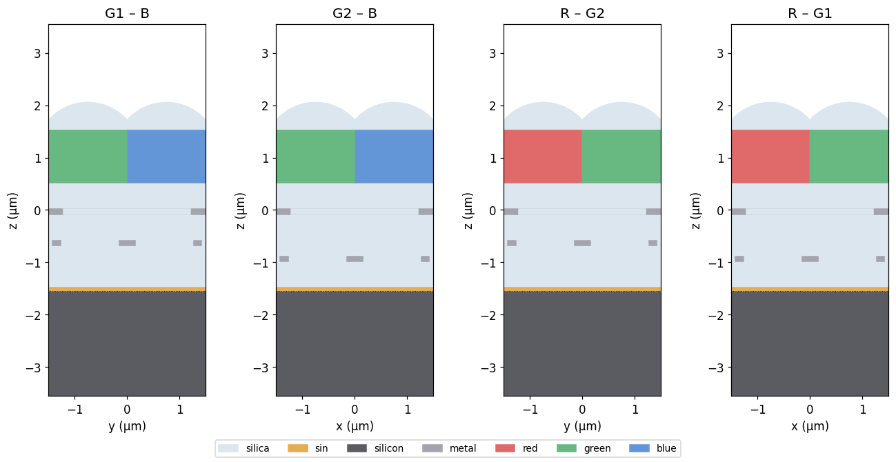
Run or load the simulation
Run the sensor and an empty cell sequentially with the JAX backend. Save the complex monitor fields, coordinates, incident spectrum, and calibrated detector efficiencies in an ignored local NumPy archive. The cache key covers both simulations and the BeamZ version. Set force_run = True after changing the solver implementation, or to repeat a calculation. The saved notebook outputs remain viewable without this local cache.
force_run = False
specs = (bz.__version__, simulation.canonical_spec(), reference_simulation.canonical_spec())
key = hashlib.sha256(pickle.dumps(specs)).hexdigest()[:16]
cache = ROOT / ".beamz_cache" / f"cmos_rgb_{key}.npz"
if force_run or not cache.exists():
    results = simulation.run(backend="jax", progress=False)
    reference = reference_simulation.run(backend="jax", progress=False)
    incident_power = -np.asarray(reference["incident_plane"].flux)
    incident_fields = reference["incident_field"]
    incident_intensity = sum(abs(incident_fields.get_dft_component(c)) ** 2 for c in ("Ex", "Ey", "Ez"))
    incident_intensity = incident_intensity.reshape(3, -1).mean(axis=1)
    assert np.all(incident_power > 0) and np.all(incident_intensity > 0)
    data = {
        "frequencies": frequencies,
        "field_wavelengths": field_wavelengths,
        "incident_power": incident_power,
        "incident_intensity": incident_intensity,
        **{pixel: -np.asarray(results[f"flux_si_{pixel}"].flux) / incident_power for pixel in pixel_signs},
    }
    for name, (_, _, axes) in planes.items():
        monitor = results[name]
        data[name] = np.stack([monitor.get_dft_component(c) for c in ("Ex", "Ey", "Ez")])
        for axis in axes:
            region = monitor.sample_region.axis_interval(axis)
            edges = results.metadata.grid.axis_edges(axis)[region.start : region.stop + 1]
            offset = results.metadata.coordinate_offset["xyz".index(axis)]
            data[f"{name}_{axis}"] = (edges - offset) / um
    cache.parent.mkdir(parents=True, exist_ok=True)
    np.savez_compressed(cache, **data)
with np.load(cache, allow_pickle=False) as saved:
    data = dict(saved)
assert all(np.isfinite(value).all() for value in data.values())
assert np.all(data["incident_power"] > 0) and np.all(data["incident_intensity"] > 0)
print(f"Monitor data: {cache.relative_to(ROOT)}")
print(f"Incident power: {data['incident_power'].min():.6f}–{data['incident_power'].max():.6f} W")
Monitor data: .beamz_cache/cmos_rgb_bee13a9c6fdc87e3.npz Incident power: 0.978523–0.988392 W
Post-run analysis
Field profiles
Plot , summing all three electric components. The denominator is the mean intensity across the empty-cell incident plane at each wavelength. Each wavelength has its own linear color bar, capped at 35% of that panel's peak to reveal weaker features. Brighter peaks saturate at the top color, indicated by the color-bar extension. Read each bar when comparing normalized intensities. Change field_vmax_fraction to adjust the display; setting it to 1 shows the full range. This changes only the visualization.
field_vmax_fraction = 0.35


def plot_rgb_fields(name, title):
    horizontal, vertical = planes[name][2]
    x, y = data[f"{name}_{horizontal}"], data[f"{name}_{vertical}"]
    intensity = (abs(data[name]) ** 2).sum(axis=0).reshape(3, len(y) - 1, len(x) - 1) / data["incident_intensity"][:, None, None]
    fig, axes = plt.subplots(1, 3, figsize=(12, 5), layout="constrained")
    for ax, values, wavelength in zip(axes, intensity, data["field_wavelengths"]):
        vmax = max(float(values.max()) * field_vmax_fraction, np.finfo(float).tiny)
        image = ax.pcolormesh(x, y, values, cmap="magma", vmin=0, vmax=vmax, shading="flat")
        ax.set(
            title=f"{wavelength * 1e9:.0f} nm",
            xlabel=f"{horizontal} (µm)",
            ylabel=f"{vertical} (µm)",
            aspect="equal",
        )
        fig.colorbar(
            image,
            ax=ax,
            label="|E|² / |E incident|²",
            shrink=0.8,
            extend="max" if field_vmax_fraction < 1 else "neither",
        )
    fig.suptitle(title)
    plt.show()


plot_rgb_fields("field_yz_BG", "G1–B sensor cross-section")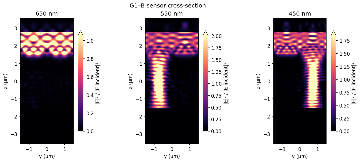
plot_rgb_fields("field_yz_GR", "R–G2 sensor cross-section")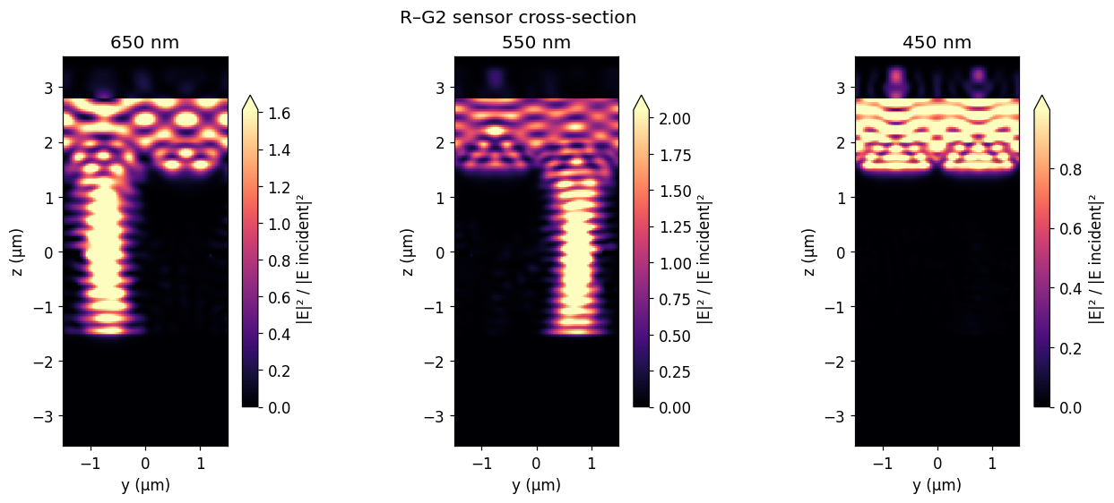
plot_rgb_fields("field_xy_silicon", "RGB fields at the silicon detector plane")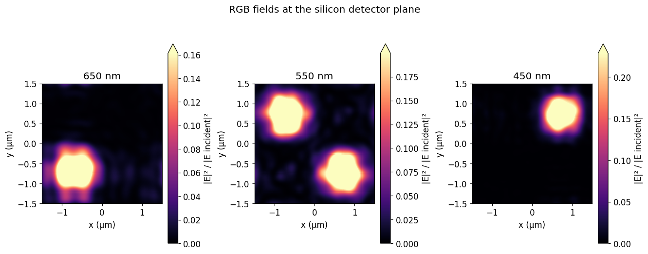
Optical efficiency
, where incident power covers the entire 3 µm × 3 µm unit cell. The saved efficiencies use the negative detector flux divided by the empty-cell incident flux at each frequency. Green sums both green apertures.
curves = {
    "red": data["red"],
    "green": data["green1"] + data["green2"],
    "blue": data["blue"],
}
wavelength_nm = bz.LIGHT_SPEED / data["frequencies"] * 1e9
order = np.argsort(wavelength_nm)
fig, ax = plt.subplots(figsize=(8, 4.5), layout="constrained")
for channel, values in curves.items():
    ax.plot(
        wavelength_nm[order],
        values[order],
        color=channel,
        lw=2,
        label="Green (G1 + G2)" if channel == "green" else channel.capitalize(),
    )
for wavelength in (450, 550, 650):
    ax.axvline(wavelength, color="gray", ls="--", lw=0.8)
ax.set(xlabel="Wavelength (nm)", ylabel="Optical efficiency", xlim=(400, 700))
ax.set_ylim(
    min(0, min(float(v.min()) for v in curves.values()) * 1.05),
    max(0.25, max(float(v.max()) for v in curves.values()) * 1.05),
)
ax.legend()
ax.grid(alpha=0.2)
plt.show()

for channel, wavelength in (("red", 650), ("green", 550), ("blue", 450)):
    value = np.interp(wavelength, wavelength_nm[order], curves[channel][order])
    print(f"{channel.capitalize():5s} at {wavelength} nm: {100 * value:.3f}%")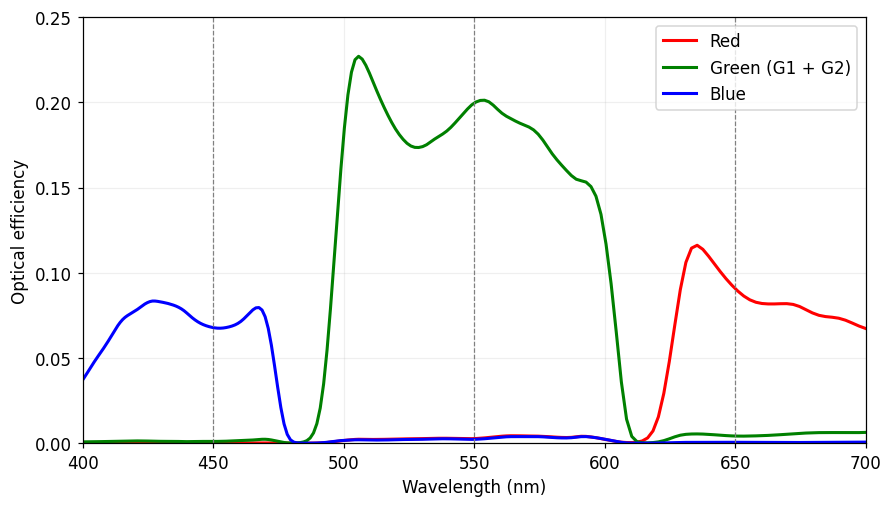
Red   at 650 nm: 9.066%
Green at 550 nm: 19.960%
Blue  at 450 nm: 6.782%
Interpretation and convergence
The field maps show how the lenses, filters, and metal stack distribute light across the pixel apertures. Optical efficiency measures power crossing those apertures, not quantum efficiency or all absorption in the silicon volume.
For quantitative use, reduce spacing, increase the absorber thickness while keeping the source outside it, and extend run_time independently until the spectra stop changing within the required tolerance.